Response / Dependent Variables
We choose to make use of “Total Engagement” as the response/ dependent variable. “Total Engagement” for each post is the sum of the total number of reactions (like, love, wow, haha, angry, sad), comments and shares of that post as of the data retrieval date. Reactions are similar to the ‘likes’ on Facebook, but provides the additional option of reacting with five animated emoji rather than a simple ‘like’ reaction.
Other possible response variables include the comment sentiment score measures, and individual engagement metrics but they are ruled out due to reasons such as their non-normal distribution and utility for our sponsor.
Explanatory / Independent Variables
Video Dataset Metadata for Analysis
| Header
|
Description
|
| Post Message Sentiment |
Crawled Variable: Sentiment Score calculated using PyCharm python script, AFINN Sentiment words and emoji package
|
| Video Duration in Seconds |
Derived Variable: The duration in seconds of the video
|
| Number of actors |
Derived Variable: Total Number of actors inside a video
|
| Video Category |
Crawled Variable: The categories of the video, 7 levels
|
| Day of Week |
Derived Variable: The time of the day from the adjusted posted column of the video, categorical 7 levels
|
| Time Interval (Hour) |
Derived Variable: The time intervals of the articles derived from recursive splitting of the hour from the time of day column, to coincide with morning, afternoon, evening and night, categorical 4 levels
|
| Video thumbnail includes Words |
Derived Categorical Dummy Variable: 1 being video thumbnail includes words and 0 being video thumbnail does not include words
|
| Video thumbnail includes Actor faces |
Derived Categorical Dummy Variable: 1 being video thumbnail includes actor faces and 0 being video thumbnail does not include actor faces
|
| Video thumbnail includes subject matter |
Derived Categorical Dummy Variable: 1 being video thumbnail includes subject matter and 0 being video thumbnail does not include subject matter
|
| Actors' names |
Derived Variable From JMP Make Indicator Columns from Actor multiresponse column. Actors that are from sponsored companies are marked as external. Actors that act in fewer than 4 videos are marked as others. There are 101 different actors
|
Data Transformation / Excluding Outliers
We have performed transformation and exclusion of outliers for the video dataset in a similar fashion as the article dataset for both the response variables and the explanatory variables.
Bivariate Fit
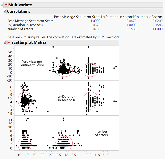
We also conduct bivariate analysis on the response variable against each transformed explanatory variable to review the linearity of fit. This step helps us to decide if the transformation of the variable is necessary, and we pick the transformation that provides the highest R2 value. The video dataset only has the three numerical variables below
Bivariate correlation scatterplot and matrix the video model
Checking for Multi-collinearity
Parameter Estimates with VIF statistics
As a result we have the list of numerical continuous explanatory variables to explain the variation of our response variables for the video regression model in preparation for the next step which is the stepwise regression.
Stepwise Regression
We proceed with the creation of our explanatory model by running stepwise regression within the Fit Model platform on JMP Pro 13 on the variables from the steps above with the inclusion of categorical variables (that will be dummy coded by JMP). We conduct a p-value threshold regression at 5% which gives the best R2 and adjusted R2 values, indicating the best model fit given the available data. We ran the regression for the forward, backward and mixed directions and realised that the R2 values for the mixed direction is the highest, and we will be using it to run our model with. AICC and BICC measures are not used since we are looking at an explanatory model instead of a predictive model.
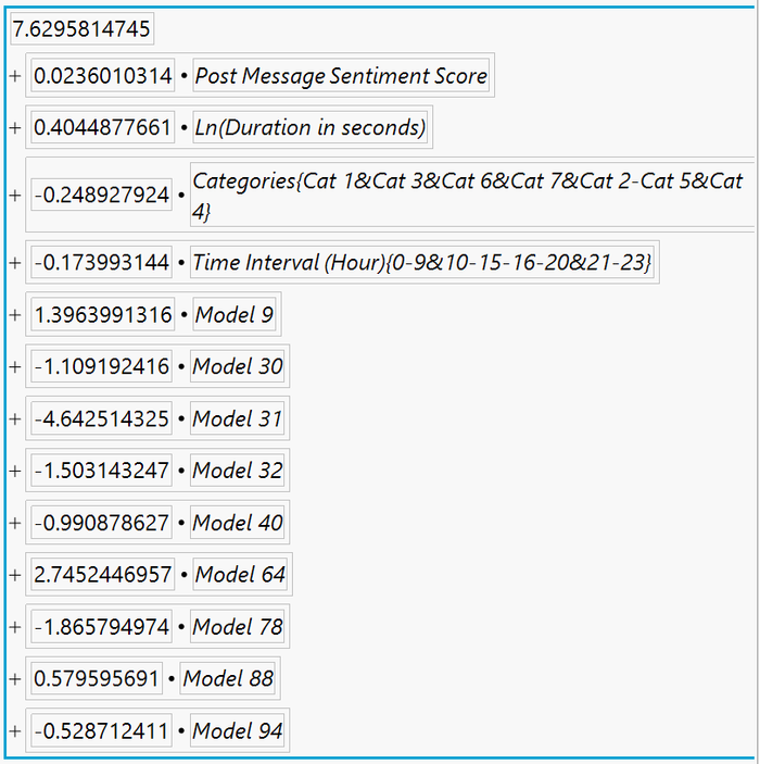
The regression equation and parameter estimates are shown below:
Video Regression equation for Ln(Total engagement)
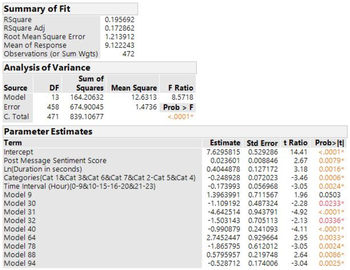
Videp Regression Parameter Estimates for Ln(Total engagement)
Model Fit and Model Assumptions
Video Regression model fit results
The goodness of fit is represented by the R2 value. R2 is a statistical measure known as the coefficient of determination which measures how close data points are to the line generated by the model.
The R2 value here for the articles model is 0.20 and represents that the variation in Ln Total Engagement for articles is 20% explained by the model.
To gauge the explanatory power of each additional explanatory variable added, we also consider the adjusted R2 value, which adjusts for the number of explanatory variables in the model – that is, it would only increase if each explanatory variable added improves the model more than what is expected by chance.
The adjusted R2 value here for the articles model is 0.17 and represents that the variation in Ln Total Engagement for articles is 17% explained by those explanatory variables that affect the response variable.
We then move on to the model assumptions to validate our regression model findings. There are several assumptions of linear regression models which need to be met, as seen below:
- Relationship between the dependent variable and independent variables is linear
- Expected mean error of the regression model is zero
- Errors/Residuals have constant variance (Homoscedastic)
- Errors/Residuals are independent of each other
- Errors/Residuals are normally distributed and have a population mean of zero
Assumption 1: Linearity
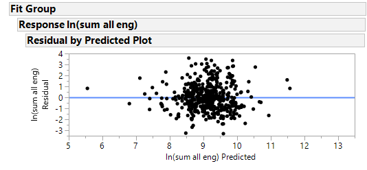
Residual by predicted plot
The points are quite symmetrically distributed around the line, and this indicates that the points are random and hence fulfills the linearity assumption.
Assumption 2: Zero expected mean error
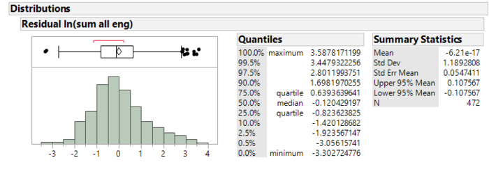
Distribution of residuals
The residuals largely follow a normal distribution with a mean close to zero and a standard deviation close to one.
Assumption 3: Homoscedasticity
Residual by predicted plot
The distribution of the points in the plot is rather symmetrical, with no signs of increasing residuals with the increase of the predicted values (it is not funnel shaped). This indicates that the residuals have constant variance and are hence homoscedastic
Assumption 4: Independent Residuals
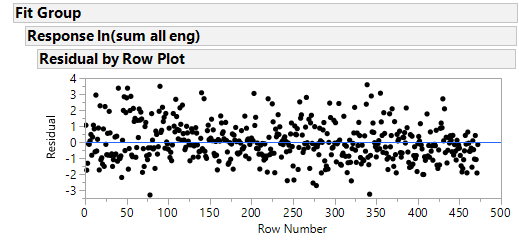
Residual by row plot
The scatter plot shows that the residuals are randomly distributed around the line and hence shows that they are time independent. This also suggests that residuals are not autocorrelated.
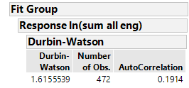
Durbin-Watson test of no autocorrelation
The Durbin-Watson d = 1.6, which is between the two critical values of 1.5 < d < 2.5. Therefore, we can assume that there is no first order linear auto-correlation in our multiple linear regression data
Assumption 5: Residuals are normally distributed
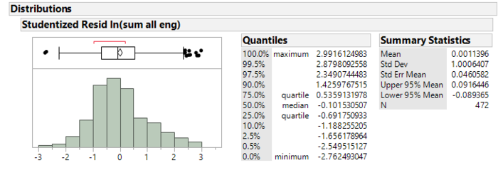
Studentized Residual distribution
The residuals largely follow a normal distribution with a mean close to zero and a standard deviation close to one, hence fulfilling this assumption.
Interpretation and Managerial insights
A multiple stepwise linear regression was run to explain Ln(Total Engagement) for video performance from post message sentiment score, Ln(duration of video in seconds), video category, hourly time interval to post and video actors. These variables statistically significantly explained Ln(Total Engagement), F(12.63, 1.47) = 8.57, p < 0.0001***, adjusted R2 = 0.17. All selected variables added statistically significantly to the explanation, p < .05. The video regression model has met all 5 assumptions highlighted above, and we believe that our sponsor can benefit from the knowledge of the determinants of their different social media engagement based on the regression equation on their video performance.
While our video explanatory regression models can explain up to 17-18% of the variation in the post’s engagement performance, insights can still be gleaned from it. Below are the points that can be drawn for the video regression model:
- Positive sounding post messages when added to the description of the video can help increase engagement.
- Video duration matters and longer videos tend to perform based on our results. However, we believe that there is an ideal video length as overtly lengthy videos could deter engagement.
- A, B, C, D, and E videos since they are significantly more popular and should place more emphasis in its content creation.
- Best time to post is in the late afternoons, evenings, and nights between 4pm to 11pm
- Actors A, B and C are performing well and can be suited for such videos whereas actors D, E, F, G, H and I do not perform that well, suggesting the need for either improvement or adjustment of assignments.
|
|
|
|
|
|
|
|
|
|
|
|
|
|
|
|
|
|
|
|
|
|
|
|

