Difference between revisions of "ISSS608 2017-18 T3 Assign Yejerla Amrutha Rajeshwari eye"
Jump to navigation
Jump to search
| Line 38: | Line 38: | ||
=<font size="5"> Now, I see </font>= | =<font size="5"> Now, I see </font>= | ||
| + | |||
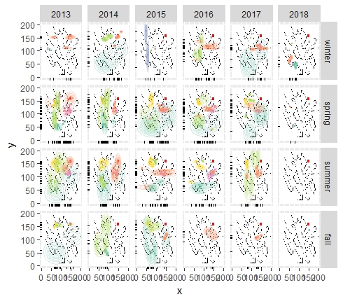
| + | Based on insights from initial exploration, the recording are further investigated with custom visualizations in R. Faceting technique is used to be able to compare observations across time frames. | ||
==='''Steps followed'''=== | ==='''Steps followed'''=== | ||
| + | #Lekagul Roadways graph is loaded on to R and after setting the axis, map is plotted on the graph using geom_raster. A rectangular geom of about 9x9 pixels is overlaid on the graph to mark the alleged dumping site. | ||
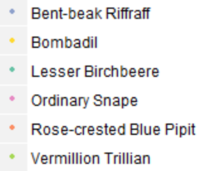
| + | #The species that we want to study further i.e. Rose Crested Blue Pipit, Bombadil, Bent beak riffraff, Lesser Birchbeere, Vermillion Trillian, Ordinary Snape are plotted on the graph. | ||
| + | #Colours of points on the graph are mapped to Species and the 2d density attribute with the same colour is added for each species. | ||
| + | #Resultant plot is faceted using a season modified_year layout | ||
| + | #Rugs are added as an visual aid. | ||
Revision as of 21:50, 8 July 2018
|
|
|
|
|
|
|
Now, I see
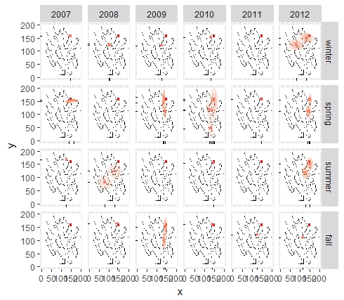
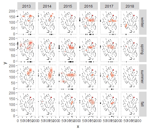
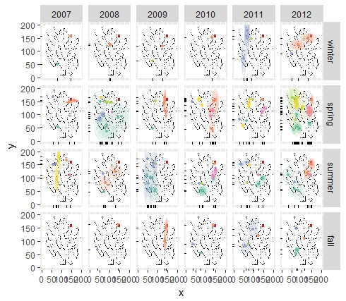
Based on insights from initial exploration, the recording are further investigated with custom visualizations in R. Faceting technique is used to be able to compare observations across time frames.
Steps followed
- Lekagul Roadways graph is loaded on to R and after setting the axis, map is plotted on the graph using geom_raster. A rectangular geom of about 9x9 pixels is overlaid on the graph to mark the alleged dumping site.
- The species that we want to study further i.e. Rose Crested Blue Pipit, Bombadil, Bent beak riffraff, Lesser Birchbeere, Vermillion Trillian, Ordinary Snape are plotted on the graph.
- Colours of points on the graph are mapped to Species and the 2d density attribute with the same colour is added for each species.
- Resultant plot is faceted using a season modified_year layout
- Rugs are added as an visual aid.
