ISSS608 2016-17 T3 Assign ONG GUAN JIE JASON Data Preparation

ISSS608 Assignment 2 Ong Guan Jie Jason

Background

Data Preparation

Visualization

Observations & Insights

Conclusion

Comments

Data Preparation

In this challenge, there are two datasets being provided. The first set contains sensor readings from air-sampling sensors that are installed within the vicinity of the four factories. The second set contains meteorological data from a weather station in proximity to the factories and sensors. Both datasets have to be cleaned and transformed before they are suitable to be imported into tableau for further analysis.

Data Description

Companies Details

This section provides a short description of the manufacturing companies near Mistford.

Roadrunner Fitness Electronics

Roadrunner produces personal fitness trackers, heart rate monitors, headlamps, GPS watches, and other sport-related consumer electronics. Roadrunner began as one of the region’s first fitness stores in 1962, with an eye toward outfitting the entire nation with appropriate outdoor gear. After an earthquake nearly destroyed their main warehouse in 1968, Roadrunner turned a bad situation into a glowing success with the first “slightly damaged goods” sale. After which they began to focus on manufacturing; though their “Earthshaking Bargains” business still sells dented, overstocked and refurbished items over the internet and from a small retail shop attached to their front office.

Kasios Office Furniture

Kasios Office Furniture manufactures metal and composite-wood office furniture including desks, tables, and chairs. Kasios wants to do with desk chairs what Starbucks did for coffee – making office furniture what people must have, instead of what they just need. “Office equipment doesn’t need to be ugly!” says founder Ken Kasios. “We have redesigned all office products to be cool, fun, and hip—even your basic stapler.” Kasios business model is focused on in-store merchandising highlighting the beauty and functionality of their “user-centered design”. They recently celebrated the one-year anniversary of a distribution and merchandising agreement with the national office supply chain store PaperKlips.

Radiance ColourTek

Radiance produces solvent based optically variable metallic flake paints. “Metallic paints with an untarnished reputation!” quips ColourTek’s Senior Vice President Arthur Donner. “Radiance ColourTek metallic paints are worth their weight in gold.” Offering a new generation of paints in the 1970s, Radiance out marketed all competitors for three decades until manufacturing process issues began to tarnish their reputation. “We were challenged,” said Donner. “Polishing up our pearlescent pigments caused us to lose luster, but now we have the lowest VOCs (volatile organic compounds) in the industry!”

Indigo Sol Boards

Indigo Sol produces skateboards and snowboards. Founder Billy Keys started off manufacturing wooden wine barrels for northwestern US wineries, but then navigated a course from decorative fiberglass wine barrels to making his first pair of fiberglass skis in 1971. Excellent product and sales decisions rocketed Keys Skis production to unexpected levels, until they were bought out by a large Denver, Colorado-based private investment group. Keys returned to making specialized snowboards in the 1980s, with a small company in Mistford called Indigo Sol. The company has seen modest growth in recent years.

Substances Details

When Mistford began growing its manufacturing industry, both the town and the companies wished to ensure an environmentally sound and economically supportive partnership. With these aims in mind, air sampling sensors have been placed near the town and in the Preserve to monitor air quality. The following substances detected are of particular concern:

Appluimonia

An airborne odor is caused by a substance in the air that you can smell. Odors, or smells, can be either pleasant or unpleasant. In general, most substances that cause odors in the outdoor air are not at levels that can cause serious injury, long-term health effects, or death to humans or animals. However, odors may affect your quality of life and sense of well-being. Several odor-producing substances, including Appluimonia, are monitored under this program.

Chlorodinine

Corrosives are materials that can attack and chemically destroy exposed body tissues. Corrosives can also damage or even destroy metal. They begin to cause damage as soon as they touch the skin, eyes, respiratory tract, digestive tract, or the metal. They might be hazardous in other ways too, depending on the particular corrosive material. An example is the chemical Chlorodinine. It has been used as a disinfectant and sterilizing agent as well as other uses. It is harmful if inhaled or swallowed.

Methylosmolene

This is a trade name for a family of volatile organic solvents. After the publication of several studies documenting the toxic side effects of Methylosmolene in vertebrates, the chemical was strictly regulated in the manufacturing sector. Liquid forms of Methylosmolene are required by law to be chemically neutralized before disposal.

AGOC-3A

New environmental regulations, and consumer demand, have led to the development of low-VOC and zero-VOC solvents. Most manufacturers now use one or more low-VOC substances and Mistford’s plants have wholeheartedly signed on. These new solvents, including AGOC-3A, are less harmful to human and environmental health.

Geo-coordinate Details

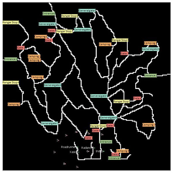
The factories and sensors locations are provided in terms of x,y coordinates on a 200x200 grid, with (0,0) at the lower left hand corner (southwest). The sensors map shows the locations of the sensors and factories by number for the sensors and by name for the factories. Some of the other features of the map (such as entrances and gates in that area) have been removed for readability. (Please note that the terms “sensor” and “monitor” are used interchangeably.)

Factories Coordinates

• Roadrunner Fitness Electronics: 89,27
• Kasios Office Furniture: 90,21
• Radiance ColourTek: 109,26
• Indigo Sol Boards: 120,22

Sensors Coordinates

• 1: 62,21
• 2: 66,35
• 3: 76,41
• 4: 88,45
• 5: 103,43
• 6: 102,22
• 7: 89,3
• 8: 74,7
• 9: 119,42

Using Excel

Sensor Data

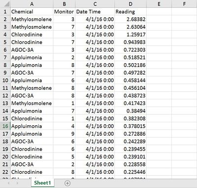
The original dataset is actually already in a very clean format which is ready to be imported into tableau. Columns are minimal and date is in a proper format with readings being reported for each sensor at an hourly fashion.

Meteorological Data

This dataset unlike the previous one requires heavy cleaning before it is ready to be imported into tableau.

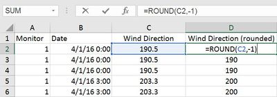
• An additional column is created to round the wind direction to the nearest tenth. For e.g., a wind direction of 190.5 degrees will be rounded to 190. This is required to make the visualization of the wind direction easier since now the wind direction varies by a fixed interval of 10 degrees.

• Each row of data will have to be replicated three times to construct a polygon to represent the wind direction at each instance of time. There will be an additional column named "point" to label the 3 points.

• A separate sheet is generated to list down the degrees starting from 10 and ending at 360. For each degree, it will be replicated 3 times again to reflect points 1-3 and the relevant degrees. For instance, a wind direction at 10 degrees will be represented by a polygon spanning from 10 to 20 degrees. Point 1 will have a length of 0 and points 2 and 3 will have a length of 1. There is an additional helper column to concatenate the degree and point to give it a unique string so that excel lookup function can be used to call the values in this sheet from the main sheet later.

• Now back to the main sheet, an additional column angle is generated to pull the values from the previous sheet via excel vlookup function. For e.g., a wind direction of 190 degrees will have to return 0 degrees, 190 degrees and 200 degrees for points 1-3 respectively.

• Also a length of 1 is too short to visualize on tableau so it is modified to 200 so that the polygon can be big enough to gain some meaningful insights later.

• The assignment states that the wind direction column reflect the direction that the wind is coming from. Thus, we will need to reflect the polygon over itself. A few additional columns have to be generated to achieve that. To start off, a column called angle between is created. As the name suggests, it is the angle in between points 2 and 3 of the polygon.
• Two more columns, degree and length1 are generated to assign the same value to each point for each wind direction at a particular date. These variables are useful for the subsequent calculations in tableau to reflect the polygon.

• Lastly, since we will be having 9 windrose plots for 9 monitors we need to multiply the current number of rows by 9 to represent the wind direction at each point of time at each monitor.

Using Tableau

Trellis Plot

Since there are 9 monitors, a total of 9 sub plots will be required. In order to do that, a row and column divider will be needed. The formula for the calculated fields are shown below:

Drag the row divider to the rows section and the column divider to the columns section. Change both measures to discrete which will be colour coded blue after it is done. Next, drag the monitor dimension into the details section. Then, right click on both the row and column divider and select compute using monitor. Now, drag the date dimension into the columns section and the readings measure into the rows section. After that, place the chemical dimension into the filter window and the trellis plot will be generated. The date dimension can be drilled down further depending on what level of aggregate measure one is interested in.

Cycle Plot

Construction of the cycle plot is relatively simple with no additional calculated fields required. Drag the date dimension into the columns section and press the plus sign beside the pill to drill down to day and hour. Next, remove the month pill and make sure the hour pill is before the day pill. Then, drag the monitor dimension and the readings measure to the rows section. Lastly, place the chemical dimension and the month dimension into the filter window.

Horizon Graph

The horizon graph is constructed on the basis of using percentiles to determine the colour intensity. The percentiles are >90%, >75%, >50% and <50%. There will be multiple calculated fields required to generate this horizon graph. First, the percentiles will need to be created and there will be a total of 5, starting from 100% and ending at 0%. The calculated field for the 100% and 90% is shown below.

Now, we want to have readings which are above the 90% have a different colour intensity so we will need a separate calculated field.

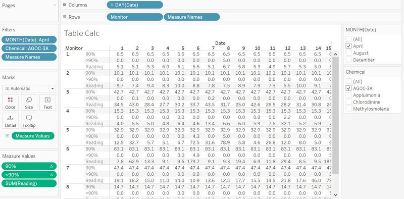
The same will calculations will have to be done for each of the percentile bracket that was defined at the start. A table calculation is generated on another sheet to make verification of the values easier.

After generating all the calculated fields required, drag the monitor dimension and measures values into the rows section. Drag the date dimension into the columns section. Then, drag the measure names into the colour window. Lastly, drag the month and chemical dimensions into the filter window.

Air Plume Model

This model is the hardest to construct out of the four. The map being used as the background image is 350 by 200 pixels. The coordinates of the monitors using the background image as reference are as follow:

1. 56, 76
2. 70, 125
3. 105, 146
4. 147, 159
5. 199, 153
6. 196, 79
7. 150, 13
8. 98, 27
9. 255, 149

First, the 9 polygons representing the 9 stream of winds that are going to be detected by the monitors need to have a corresponding x and y axis to be represented on the map. There will be 1 calculated field for the x-axis but 10 calculated fields for y-axis 1-9. The last y-axis will be used to align the background image to the height required.

The rest of the y-axis calculated fields will be largely similar with the addition of the initial y coordinate of each monitor being different.

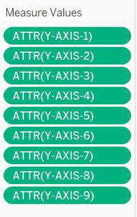
Now drag the x-axis measure into the columns section and the y-axis measure into the rows section. Then, drag the measures value into the rows section as well and retain only y-axis 1-9 in the window. Change the measure values into dual axis.

Drag the point measure into the path window and wind direction, wind speed and monitor into the details window. Lastly, drag the month and monitor dimensions into the filter window.