ANLY482 AY2017-18T2 Group01: Project Management
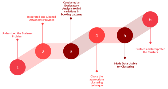
We went through the following steps to execute our project:
We first wanted to gather all information related to the booking journey of customers and the key influencing factors. To do this we carried out the following steps:
1. Spoke with eatigo employees beyond our sponsor (Sales Lead and Marketing Lead)
2. Interviewed eatigo customers to understand their typical priorities and their customer journey.
Based on our understanding, we have mapped out the customer journey map as follows:
The next step involved zooming into the data sheets provided to us and understand each variable, it's sufficiency and relevance in helping us solve the business problem, and then preparing it for analysis. These were the steps in Data Preparation:
The details of our work in each step has been summarized as follows:
After this, we conducted an exploratory data analysis. However, due to confidentiality reasons, we are not detailing the visualizations. If required, please free to contact us for more information [(Contact Details)]
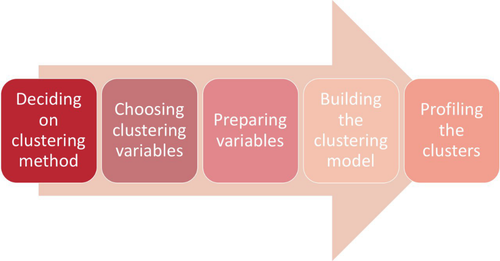
We followed the following method for our Clustering:
Literature Review:
As has been described in literature repeatedly, an important part of clustering is choosing an appropriate clustering method. Aldenderfer and Blashfield [1], in their book about clustering, explore and compare different methods of clustering like K-Means (partition based) clustering and Hierarchical Methods of Clustering. K-Means Clustering partitions n observations into k clusters in which each observation belongs to the cluster with the nearest mean. On the other hand, Hierarchical Clustering starts by treating each observation as a separate cluster and repeatedly groups observations until all clusters merge together. One of the key takeaways from the book is that "Although the strategy of clustering may be structure-seeking, its operation is one that is structure-imposing." Thus, one must be very meticulous in choosing an appropriate clustering method well-suited for the data.
Rajagopal [2], in his study to identify high-profit, high-value and low-risk customers for large companies uses a demographic clustering algorithm. Through his process, he notes that K-Means clustering technique is more appropriate for clustering a large dataset due to the low computational requirements of the method. It is especially efficient when there are many variables included in the analysis. However, he also notes that it is a greedy solution and may not always reach the global optimal solution as it is highly reliant on the initial seeds.
The paper by Oyelade, Oladipupo and Obagbuwa [3] describes an instance of K-means clustering to analyze student's results data and create clusters of students which are not only based on GPA. The authors choose the K-Means algorithm because of its ease and simplicity of implementation, scalability, speed of convergence and adaptability to sparse data. Though we have a much larger data set, we were certain that our client requires a scalable and fast solution as well. However, unlike Oyelade, Oladipupo and Obagbuwa [3] our clustering does not include demographic variables.
Customer segmentation has also been a common topic of research. Wu and Chou [4], perform a clustering for an ecommerce company using a soft-clustering approach. They recognize that RFM (recency, frequency and monetary) variables are key drivers towards creating their clusters. Thus, though we have chosen K-Means in our analysis, we have also used such variables such that are clusters are of value to the company.
Choosing the Clustering Method:
Based on our understanding of the literature and in consultation with our sponsor and supervisor, we decided on K-Means clustering as the appropriate clustering technique because of the following reasons:
i) K-means clustering is suitable for large data sets
ii) K-means is less affected by outliers and presence of irrelevant variables
How K-Means Works
K-means algorithm is a kind of data partitioning method used for clustering. K stands for the number of clusters and the algorithm identifies clusters their means. K means clustering works on the fundamental concept of Euclidean distance. Euclidean distance is a distance measure based on the location of points in the space. A distinction can be made here from Non-euclideanNon-Euclidean distances which is based on properties of point in a space.
Like other clustering algorithms, the ultimate aim of K means clustering is to group objects in such a way that the they are homogenous within a cluster and heterogenous across clusters . This it ensures by minimizing within cluster variation. K means clustering is an iterative process. It starts by randomly assigning objects to a pre-specified number of clusters based on Euclidean distance of the points from the cluster centers or centroids. In the iterations that follow, objects are reassigned to other clusters so as to minimize the within cluster variation. If the reassignment of an object reduces the within cluster variation, that object is reallocated to that cluster.
1. Initialize:
Pre-specify the number of clusters and arbitrarily choose objects as cluster centres. Let clusters be represented by k=1,2,…,K. This is the 0th iteration i.e. h=0
2. Assign Clusters:
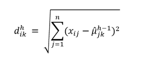
Assign object i to cluster k: the cluster with the closest mean based on Euclidean distance. The Euclidean distance between object i and cluster mean μ_k^h in iteration h is calculated as:
Where j=1,…,n represents the clustering variables. Object i is assigned to the cluster to satisfy the following:
The argument ensures that the Euclidean distance from the object,i to the group g, is minimized
3. Compute Cluster Means:
With the fixed cluster assignments calculate the cluster means for each of the variables
Therefore, the new estimate of cluster mean is the simple average of all observations assigned to it.
4. Compute SSE
Sum of Squared Errors (SSE) measures the total within cluster variations. The error gives distance between each observation and its closest cluster mean.
5. Loop:
The steps from Step 2 onwards are repeated to reassign objects to clusters by comparing the Euclidean distance across clusters. Since the cluster centres’ positions keep changing with each iteration, the clustering solution keeps changing as well. This is done until the convergence criterion is satisfied. Convergence criterion is usually that there is no change in cluster affiliations i.e. change in SSE is small.
Data Preparation for K-Means
1. Integrating the Data Sets
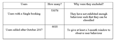
To decide on which variables would be appropriate for clustering we relied on data availability and intuition. We used the integrated data sheet to extract the 136,177 users and variables that would be most relevant to our clustering. JMP Pro was used to then create a clustering data sheet – first, separate tables were created for each variable by grouping the data by User ID and then the tables were joined together by matching User ID. This sheet was further filtered to exclude the following set of users:
After filtering, the clustering sheet consists of 78,483 user records with each row representing a unique user and each column corresponding to variables that represent users’ characteristics.
2. Preparing Variables
Step 1: Variable Creation
New variables: To segment customers along the Recency, Frequency and Monetary (RFM) dimensions, we created appropriate variables using the data available to us. We also created variables which will allowed us to classify users based on their variety seeking behaviour when it comes to restaurants and cuisines. These are shown below:
Step 2: Converting Categorical Variables into Continuous
Most of the variables in our dataset are categorical variables such as Booking Discount (10-15, 20-25, 30-35, 40-45, 50) Restaurant Tier (Tier 1, Tier 2, Tier3, Tier 4, Tier 5) etc. As discusses earlier, K-means uses cluster means to calculate the Euclidean distance. Since, means is not the central tendency measure for categorical variables, K-means algorithm cannot be applied to categorical variables in their raw form to perform clustering.
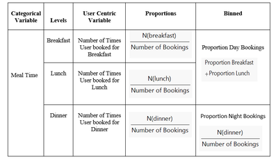
Therefore, we first converted categorical variables into user-centric continuous variables by splitting the variables into its different levels and then calculated them as proportions (by dividing by total number of bookings) to make the variables more meaningful for clustering. For some of the categorical variables such as Tier and Meal Time, one level dominated the others and therefore proportions were binned to ensure that the variables will sufficiently differentiate the segments. [5] An example of how we treated categorical variables is shown below:
Step 3: Tests for Collinearity
A high correlation amongst clustering variable can lead to misrepresentation of clusters since the variables are not sufficiently unique to identify different clusters. If variables are highly correlated (~90%), aspects of these variables will be overrepresented as the clustering technique will not be able to differentiate between the variables. To avoid perfect multicollinearity, we excluded one level for each categorical variable. For example, for booking day split into weekday and weekend, only weekday was used as an input variable in a conceptual sense. Therefore, we first ran a MANOVA (Multivariate Analysis of Variance) test on JMP Pro, to check for correlation amongst our variables and obtained the following results:
From the output we see that no two different variables exhibit a very high correlation and therefore are suitable for clustering in this respect.
Step 4: Checking for Skewness and Variables Transformation
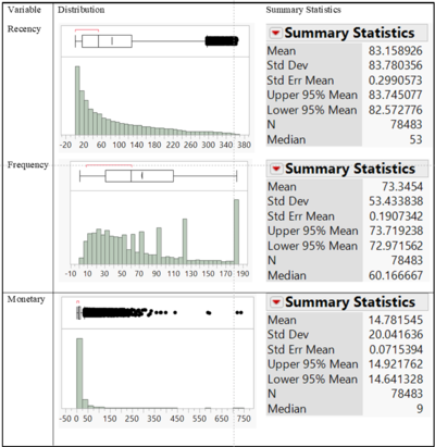
As the next step, we mapped out the variable distributions to check for outliers and skewness in the variables. In the variable distributions, the X axis represents the range of the variable and the height of the bars represent the number of users.
We confirmed with our sponsor about the outliers and did not remove them to avoid misrepresentation of user behaviour. As for skewness, most of our variables were right skewed or positively skewed i.e. the mean was greater than the median. Since it is integral to remove skewness and normalize the data before inputting into the K-means algorithm, we used the Johnson transformation to transform our variables’ distribution to normal distributions. The Johnson system of transformations has the general form of
Where the transformation function is represented by f, γ and δ represent the shape parameters that are determined by the skewness and kurtosis of the variable, λ and ξ represent the the mean and standard deviation respectively. Before going ahead with the Johnson transformation, we tried log, square root and a global transformation method. However, these methods were not effective in normalizing all our variables and therefore we went ahead with the Johnson transformation which caters to each variable separately and uses the form that best transforms that variable.
Performing the Clustering
Step 1: Deciding on the Number of Clusters
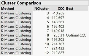
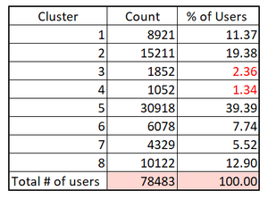
As established earlier, K-means algorithm requires the researcher to pre-decide on the number of clusters or the value of k. However, choosing too small a k value can lead to overfitting and over generalization with a cluster comprising of too many observations. At the same time, choosing a very large value for k may lead to clusters that are too small without any defining characteristics. Therefore, to strike a balance between the two, we implemented clustering in ranges, going from a smaller range (3-6) to a larger range (3-15) in increments of 1. Through a process of elimination, we found k = 8 clusters to be the most optimal having the largest ‘CCC’ score and the fewest number of clusters with less than 5% of total users. CCC refers to the Cubic Clustering Criterion and measures the fit of the clustering model. The CCC value is calculated by comparing the R squared value one would obtain if objects were grouped according to the specified K value (Cluster k ) versus the R squared one would obtain from a hypercube of uniformly distributed random points together with the points in a cluster (Cluster k + random points).The CCC values can either be negative or positive. If, for the specified range, all of the k values have a corresponding CCC value that is negative, perhaps, something is wrong with the data set and the researcher must then review the data preparation method. A larger CCC value indicates a better fit.
The output is shown below:
JMP Pro uses the CCC or cubic Clustering Criterion Method to determine the optimal number of clusters.
Step 2: Profiling the Clusters
Profiling Technique: Z-score Method
Profiling or characterizing clusters involves giving a meaningful interpretation to the clusters. The following things must be kept in mind while developing cluster profiles:
- What are the characteristics common to objects within a cluster?
- What are the characteristics unique to the cluster?
There are several techniques that can be used for this purpose. One such technique is the Z-score profiling method. We used the Z-score profiling technique to profile our clusters since the Recency, Frequency, Monetary variables are measured on a different scale than proportions making comparison difficult. The Z-score method circumvents this problems by standardizing values such that negative z-scores are interpreted as being x standard deviations below the 0 mean and positive z-scores are interpreted as being x standard deviations above the 0 mean. The magnitude x of the z-score value indicates the distance between mean 0 and z-score value. A more extreme magnitude of Z-score represents a larger deviation from the 0 mean and therefore a stronger preference for or against that dimension. JMP allows the user to save the clusters to the data table such that each object has a cluster number assigned to it. The user can then obtain the cluster means, population means and population standard deviations which are inputs in the Z-score formula. The Z- score is calculated as:
Where Z(kj) is the z-score for cluster k=1,…,8 for variable j. Cluster Mean (kjis) the mean for variable j for cluster k, Population Mean (j) is the variable mean across the entire population and Population Standard Deviation (j)is the variable standard deviation across the entire population. The cluster means before converting into z-scores are shown in the table below:
Interpreting the User Segments
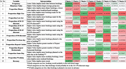
Based on the method described in the previous section, we conducted a z-score profiling on the 8 clusters we had generated and found the following Z-Score Results. The colour gradient represents the relative value across the 8 Clusters. To profile the clusters, we sorted the Z-scores such that the extreme values give us an indication of the identifying characteristics of the user segment. We then compared the Z-scores across clusters to gauge an idea of where a cluster stands with respect to other clusters along the variable under consideration.
We were able to create 7 Distinct Customer Clusters. For a more detailed breakdown of this, please refer to the [Project Findings ] page.
Just a note, while interpreting the cluster outputs, we factored in some general understanding of the business. Knowing that 50% discounts are generally available for off-peak periods, we have inferred that the customers who use this discount tier more are more committed to the eatigo platform. Further, when we combine this with their restaurant tier preference, we believe that those who tend to book higher tiered restaurants at higher discounts, really maximise the use of the eatigo platform.
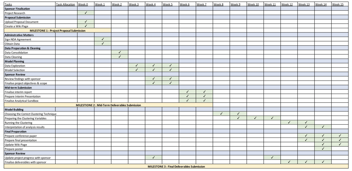
We followed the work plan below to ensure we met the deadlines of this project
References:
[1] M. Aldenderfer and R. Blashfield, Cluster Analysis. 2455 Teller Road, Thousand Oaks California 91320 United States of America: SAGE Publications, Inc., 1984.
[2] D. S. Rajagopal, E. DW, and B. Consultant, "CUSTOMER DATA CLUSTERING USING DATA MINING TECHNIQUE," Int. J. Database Manag. Syst., p. 11, 2011.
[3] O. J. Oyelade, O. O. Oladipupo, and I. C. Obagbuwa, "Application of k-Means Clustering algorithm for prediction of Students' Academic Performance," IJCSIS Int. J. Comput. Sci. Inf. Secur., vol. 7, no. 1, 2010.
[4] R.-S. Wu and P.-H. Chou, "Customer segmentation of multiple category data in e-commerce using a soft-clustering approach," Electron. Commer. Res. Appl., vol. 10, no. 3, pp. 331-341, May 2011.
[5] M. Sarstedt and E. Mooi, "Cluster Analysis," in A Concise Guide to Market Research, Springer, Berlin, Heidelberg, 2014, pp. 273-324.
[6] P.-N. Tan, M. Steinbach, and V. Kumar, Introduction to data mining. Boston : Pearson/Addison Wesley.
[7] F. George, "Johnson's system of distributions and microarray data analysis," p. 99.
[Our discussions with the sponsor, professor and amongst ourselves ]
