Social Media & Public Opinion - Final
Contents
Change in project scope
Having consulted with our professor, we have decided to shift our focus away from developing a dashboard and delve deeper into the subject of text analysis of social media data, specifically Twitter data. Social media has changed the way how consumers provide feedback to the products they consume. Much social media data can be mined, analysed and turned into value propositions for change in ways companies brand themselves. Although anyone and everyone can easily attain such data, there are certain challenges faced that can hamper the effectiveness of such analysis. Through this project, we are going to explore what some of these challenges are and ways in which we can overcome them.
Methodology: Text analytics using RapidMiner
Download RapidMiner here
| Screenshots | Steps |
Setting up RapidMiner for text analysisTo carry out text processing in RapidMiner, we need to download the plugin required from the RapidMiner's plugin repository. Click on Help > Managed Extensions and search for the text processing module. Once the plugin is installed, it should appear in the "Operators" window as seen below. | |
| |
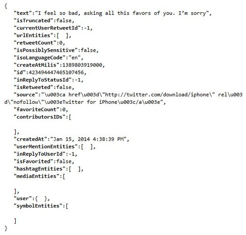
Data PreparationIn RapidMiner, there are a few ways in which we can read a file or data from a database. In our case, we will be reading from tweets provided by the LARC team. The format of the tweets given was in the JSON format. In RapidMiner, JSON strings can be read but it is unable to read nested arrays within the string. Thus, due to this restriction, we need to extract the text from the JSON string before we can use RapidMiner to do the text analysis. We did it by converting each JSON string into an javascript object and extracting only the Id and text of each tweet and write them onto a comma separated file (.csv) to be process later in RapidMiner. |
Defining a Standard
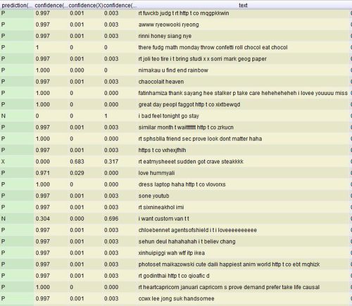
Before we can create a model for classifying tweets based on their polarity, we have to first define a standard for the classifier to learn from. In order to attain such a standard, we manually tag a random sample of 1000 tweets with 3 categories; Positive (P), Negative (N) and Neutral (X) through a mutual agreement between the 3 of us. One of the challenges faced is understanding irony as even humans sometimes face difficulty understanding someone who is being sarcastic. It is proven in a University of Pittsburgh study that humans can only agree on whether or not a sentence has the correct sentiment 80% of the time.[1]
With the tweets and their respective classification, we were ready to create a model for machine learning of tweets' sentiments.
Creating a Model
| Screenshots | Steps |
| |
| |
| |
| |
| |
|
1. Tokenizing the tweet by word Tokenization is the process of breaking a stream of text up into words or other meaningful elements called tokens to explore words in a sentence. Punctuation marks as well as other characters like brackets, hyphens, etc are removed. 2. Converting words to lowercase All words are transformed to lowercase as the same word would be counted differently if it was in uppercase vs. lowercase. 3. Eliminating stopwords The most common words such as prepositions, articles and pronouns are eliminated as it helps to improve system performance and reduces text data. 4. Filtering tokens that are smaller than 3 letters in length Filters tokens based on their length (i.e. the number of characters they contain). We set a minimum number of characters to be 3. 5. Stemming using Porter2’s stemmer Stemming is a technique for the reduction of words into their stems, base or root. When words are stemmed, we are keeping the core of the characters which convey effectively the same meaning. Porter Stemmer vs Snowball (Porter2)[2] Porter: Most commonly used stemmer without a doubt, also one of the most gentle stemmers. It is one of the most computationally intensive of the algorithms(Granted not by a very significant margin). It is also the oldest stemming algorithm by a large margin. Snowball (Porter2): Nearly universally regarded as an improvement over porter, and for good reason. Porter himself in fact admits that Snowball is better than his original algorithm. Slightly faster computation time than snowball, with a fairly large community around it. We use the Porter2 stemmer. | |
| |
| |
| |
| |
|
Improving accuracy
One of the ways to improve the accuracy of the model is to remove words that do not appear frequently within the given set of documents. By removing these words, we can ensure that the resulting words that are classified are mentioned a significant number of times. However, the challenge is to determine what the number of occurrences required is before a word can be taken into account for classification. It is important to note that the higher the threshold, the smaller the result and word list would be. Practical problems exist when modeling text statistically, since we require a reasonably sized corpus in order to overcome sparseness problems, but at the same time we face the challenge of irrelevant words exerting their weights on an independent set of test data when applying the model
We experimented with multiple values to determine the most appropriate amount of words to be pruned off, bearing in mind that we need a sizeable number of words with a high enough accuracy yield.
- Percentage pruned refers to the words that are removed from the word list that do not occur within the said amount of documents. e.g. for 1% pruned out of the set of 1000 documents, words that appeared in less than 10 documents are removed from the word list.
| Percentage Pruned | Percentage Accuracy | Deviation | Size of resulting word list |
|---|---|---|---|
| 0% | 39.3% | 5.24% | 3833 |
| 0.5% | 44.2% | 4.87% | 153 |
| 1% | 42.2% | 2.68% | 47 |
| 2% | 45.1% | 1.66% | 15 |
| 5% | 43.3% | 2.98% | 1 |
From the results, we could infer that a large number of words (3680) appears only in less than 5 documents as we see the resulting size of the word list falls from 3833 to 153 when we set the percentage pruned at 0.5%
Deriving word associations from tweets
Modeling words co-occurrence is important for many natural language applications, such as topic segmentation (Ferret, 2002), query expansion (Vechtomova et al., 2003), machine translation (Tanaka,2002), language modeling (Dagan et al., 1999; Yuret, 1998), and term weighting (Hisamitsu andNiwa, 2002). We want to know if certain words given within a set of tweets happens more often than expected by chance.
Creating word Associations with rapidminer
| |
| |
|
With tweets holding at most a 140 characters, it is no surprise that we are unable to derive high volumes of word associations from the data set. It is even harder to derive word associations when the data set is time-based rather than event-based. The topics discussed varies greatly, making it hard to formulate word associations
Pitfalls of using conventional text analysis on social media data
Multiple languages
Misspelled words and abbreviations
Length of status
Other media types
Improving the effectiveness of sentiment analysis of social media data
Allowing the user to tag their feelings to their status
One of the ways in which Facebook may make such analysis easier is by allowing the user to specify how he/she is feeling at the moment of posting a status. With this option, Facebook has effectively increase the probability of determining the right sentiment of the user at the point in time. This mitigates the possibility of sarcasm or other inferred sentiments within that post itself
Analyse data on an event/topic basis rather than on time
The data that we used was from all of the tweets by registered users with LARC in Singapore, within a given time frame of 1 month. Drilling down this tweets to a particular topic (hashtag) or an event would bring about more significant results.
Future extension
References
- ↑ Wiebe, J., Wilson, T., & Cardie, C. (2005). Annotating Expressions of Opinions and Emotions in Language. Language Resources and Evaluation, 165-210. Retrieved from http://people.cs.pitt.edu/~wiebe/pubs/papers/lre05.pdf
- ↑ Tyranus, S. (2012, June 26). What are the major differences and benefits of Porter and Lancaster Stemming algorithms? Retrieved from http://stackoverflow.com/questions/10554052/what-are-the-major-differences-and-benefits-of-porter-and-lancaster-stemming-alg


