Social Media & Public Opinion - Final

HOME

TEAM

PROJECT OVERVIEW

FINDINGS

PROJECT MANAGEMENT

DOCUMENTATION

Proposal

Final

Change in project scope

Having consulted with our professor, we have decided to shift our focus away from developing a dashboard and delve into the subject of text analysis of social media data, or Twitter data. Social media has changed the way how consumers provide feedback to the products they consume. Much social media data can be mined, analysed and turn into value propositions for change in ways companies brand themselves. Although anyone and everyone can easily attain such data, there are certain challenges faced that can hamper the effectiveness of analysis. Through this project, we are going to see what are some of these challenges and way in which we can overcome them.

Methodology: Text analytics using Rapidminer

Setting up Rapidminer for text analysis

Download Rapidminer from here

	Steps
	To do text processing in Rapidminer, we will need to download the pluging from the Rapidminer's plugin repository. Click on Help > Managed Extensions and search for the text processing module. Once the plugin is installed, it should appear in the "Operators" window as seen below.
	Data Preparation In Rapidminer, there are a few ways in which we can read a file or data from a database. In our case, we will be reading from the Tweets provided by the LARC team. The format of the tweets given were in the JSON format. In Rapidminer, JSON strings can be read but it is unable to read nested arrays within the string. Thus, due to this restriction, we need to extract the text from the JSON string before we can use Rapidminer to do the text analysis. We did it by converting each JSON string into an javascript object and extracting only the Id and text of each tweet and write them onto a comma seperated file(.csv) to be process later in Rapidminer.

Defining a standard

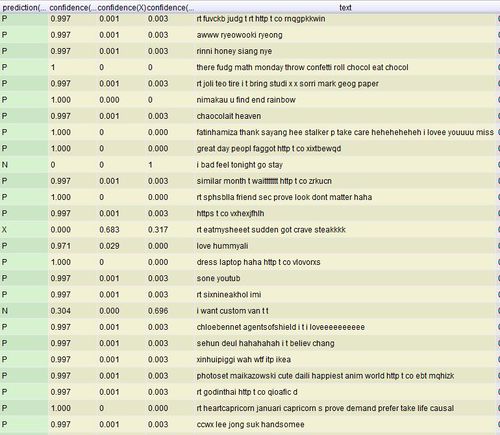
Before we can create a model for classifying tweets based on their polarity, we have to first define a standard for the classifier to learn from. To attain this standard, we manually tag a random sample of 1000 tweets with 3 categories; Positive (P), Negative (N) and Neutral (X).

With the tweets and their respective classification, we were ready to create a model for machine learning of tweets sentiments.

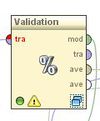
Creating the model

	We first used the "read CSV" operator to read the text from the prepared CSV file that was done earlier. This can be done via an "Import Configuration Wizard" or set manually.
	Each column is separated by a "," Trim the lines to remove any white space before and after the tweet Check the "first row as names" if there a ehader is specified
	To check on the results at any point of the process, right click on any operators and add a breakpoint. To process the document, we will need to convert the data from norminal to text.
	We will need to convert the text data into documents. In our case, each tweet will be converted in a document.
	The "process document" operator is a multi step process to break down each document into single words. The number of frequency of each word, as well as their occurrences (in documents) will be calculated and used when formulating the model. To begin the process, double click on the operator.
	1.Tokenizing the tweet by word Tokenization is the process of breaking a stream of text up into words or other meaningful elements called tokens to explore words in a sentence. Punctuation marks as well as other characters like brackets, hyphens, etc are removed. 2.Converting words to lowercase All words are transformed to lowercase as the same word would be counted differently if it was in uppercase vs. lowercase. 3.Eliminating stopwords The most common words such as prepositions, articles and pronouns are eliminated as it helps to improve system performance and reduces text data. 4.Filtering tokens that are smaller than 3 letters in length Filters tokens based on their length (i.e. the number of characters they contain). We set a minimum number of characters to be 3. 5.Stemming using Porter2’s stemmer Stemming is a technique for the reduction of words into their stems, base or root. When words are stemmed, we are keeping the core of the characters which convey effectively the same meaning. We use the default go-to Porter stemmer.
	Return to the main process. We will need to add the "Set Role" process to indicate the label for each tweet. We have a column called "Classification" and we will be assigning that column to be the label.
	The "X-validation" operator will now create a model based on our manual classification which can later be used on another set of data. To begin, double click on the operator.
	We will do a X-validation using the Naive Bayes model classification, a simple probabilistic classifier based on applying Bayes' theorem (from Bayesian statistics) with strong (naive) independence assumptions. In simple terms, a Naive Bayes classifier assumes that the presence (or absence) of a particular feature of a class (i.e. attribute) is unrelated to the presence (or absence) of any other feature. The advantage of the Naive Bayes classifier is that it only requires a small amount of training data to estimate the means and variances of the variables necessary for classification. Because independent variables are assumed, only the variances of the variables for each label need to be determined and not the entire covariance matrix. The input dataset is partitioned into k subsets of equal size. Of the k subsets, a single subset is retained as the testing data set (i.e. input of the testing subprocess), and the remaining k − 1 subsets are used as training data set (i.e. input of the training subprocess). The cross-validation process is then repeated k times, with each of the k subsets used exactly once as the testing data. The k results from the k iterations then can be averaged (or otherwise combined) to produce a single estimation. The value k can be adjusted using the number of validations parameter. Increasing the number of k will improve performance on the training data, but not necessarily on an independent set of data. This is called 'over-fitting'. The Cross-Validation operator predicts the fit of a model to a hypothetical testing data.
	To apply this model to a new set of data, we will repeat the above steps of reading a CSV file, converting it the input to text, set the role and processing each document before applying the model to the new set of tweets.
	From the performance output, we achieved a 44.6% accuracy when the model was cross validated with the original 1000 tweets that were manually tagged. To affirm this accuracy, we randomly extracted 100 tweets from the fresh set of 5000 tweets and manually tag these tweets and cross validated with the predicted values by the model. The predicted model did in fact have an accuracy of 46%, a close percentage to the 44.2% accuracy using the X-validation module.

Improving accuracy

One of the ways to improve the accuracy of the model is to remove words that does not appear frequently within the given set of documents. By removing these words, we can ensure that the resulting words that are classified are mentioned a significant number of times. However, the challenge would be to determine what is the number of occurrences required before a word can be taken into account for classification. It is important to note that the higher the threshold, the smaller the resultant word list would be.

We experimented with multiple values to determine the most appropriate amount of words to be pruned off, bearing in mind that we need a sizeable number of words with a high enough accuracy yield

• Percentage pruned refers to the words that are removed from the wordlist that do not occur within the said amount of documents. eg. for 1% pruned out of the set of 1000 documents, words that appeared in less than 10 documents are removed from the wordlist.

Percentage Pruned	Percentage Accuracy	Deviation	Size of resulting word list
0%	39.3%	5.24%	3833
0.5%	44.2%	4.87%	153
1%	42.2%	2.68%	47
2%	45.1%	1.66%	15
5%	43.3%	2.98%	1

From the results, we could infer that a large number of words (3680) appears only in less than 5 documents as we see the resulting size of the word list falls from 3833 to 153 when we set the percentage pruned at 0.5%

Pitfalls of using conventional text analysis on social media data

Multiple languages

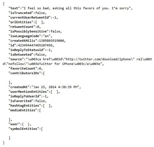
Misspelled words and abbrevations

Length of status

Other media types

Improving the effectiveness of sentiment analysis of social media data

Allowing the user to tag their feelings to their status

One of the ways in which Facebook may make such analysis easier is by allowing the user to specify how he/she is feeling at the moment of posting a status. With this option, Facebook has effectively increase the probability of determining the right sentiment of the user at the point in time. This mitigates the possibility of sarcasm or other inferred sentiments within that post itself

Limitations & Assumptions

Limitations	Assumptions
Insufficient predicted information on the users (location, age etc.)	Data given by LARC is sufficiently accurate for the user
Fake Twitter users	LARC will determine whether or not the users are real or not
Ambiguity of the emotions	Emotions given by the dictionary (as instructed by LARC) is conclusive for the Tweets that is provided
Dictionary words limited to the ones instructed by LARC	A comprehensive study has been done to come up with the dictionary

Future extension

• Scalable larger sets of data without hindering on time and performance
• Able to accommodate real-time data to provide instantaneous analytics on-the-go

Acknowledgement & credit

• Dodds PS, Harris KD, Kloumann IM, Bliss CA, Danforth CM (2011) Temporal Patterns of Happiness and Information in a Global Social Network: Hedonometrics and Twitter. PLoS ONE 6(12)
• Companion website: http://hedonometer.org/
• Schwartz HA, Eichstaedt J, Kern M, Dziurzynski L, Agrawal M, Park G, Lakshmikanth S, Jha S, Seligman M, Ungar L. (2013) Characterizing Geographic Variation in Well-Being Using Tweets. ICWSM, 2013
• Helliwell J, Layard R, Sachs J (2013) World Happiness Report 2013. United Nations Sustainable Development Solutions Network.
• Bollen J, Mao H, Zeng X (2010) Twitter mood predict the stock market. Journal of Computational Science 2(1)
• Happy Planet Index

References