Final Progress
| Mid-Term Progress
|
Final Progressnew! |
| No | Final Deliverables |
|---|---|
| 01 | Final Conference Paper |
| 02 | Final Presentation Slides |
| 03 | Final Poster |
An excerpt from the Final Conference Paper is shown below. For more information on the complete analysis, please download the paper or contact the team.
The healthcare industry in Singapore has always been keen on gathering insights on patients and their no-show appointments at their clinics. Hospitals are adopting a multi-pronged approach in reducing no-show appointments by improving the efficiency of appointment system and enabling patients to make changes of appointments more easily. The number of no-show appointments has an impact on the operational costs and clinic utilization. It also presents an opportunity cost for another patient who is unable to make use of the no-show appointment slot to get a consultation from a doctor or an allied health professional. In this study, we aim to identify significant factors that affect no-show appointments in a hospital. Taking references from past literature review, we will select and derive relevant variables to be used for modelling a possible solution for the problem being studied. We will develop models to predict the probability of no-shows for a hospital using both patient information and individual clinical appointment attendance records. We will then compare the different models and assess the results.
Based on our findings, we will end the report with set of implications and results for a hospital.
With regards to the state of mental health disorders in children, there has been an increase of cases from 533 in 1980 to 3051 in 2010. A medical study (Woo, et al, 2007) has shown that one in eight children in Singapore has emotional disorders, and one in 20 has behavioural disorders, only 10% ever see a psychiatrist. Thus, it places an emphasis in understanding no- show appointments. Appointments are made for a reason. When patients default on their appointments, they miss the opportunity for a medical consultation and thus, place their health status at risk.
No-show appointment is defined as when a patient does not attend for a scheduled clinic appointment or cancels with such minimal lead time that the slot cannot be filled (Huang & Hanauer, 2014). The impact of no-show appointments includes disruption of efficient operations of the clinics, provider productivity, decreased access to care and depriving other patients of the opportunity to see a medical professional during no-show appointments.
Hospital X is a pioneer tertiary hospital that provides a comprehensive range of medical and rehabilitative services for children, adolescents, adults and the elderly. Patients are usually referred to Hospital X by other medical institutions or they booked an appointment directly. Patients can be categorised according to their appointments with a doctor, an allied health professional or even both.
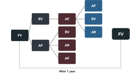
A patient’s first appointment begins with a diagnosis by a doctor and subsequent appointments are made according to the patient’s mental health status. If a patient does not have any appointment for a year, any subsequent appointment will have to be diagnosed by a doctor again (FV).
Our project sponsor is a medical consultant working for Hospital X. He specialises in tending to younger patients from the age of 18 years old and below. He hopes to tap into the under-utilised administrative data that is collected by the hospital daily.
According to our project sponsor, Hospital X experiences high no-show appointments rate of about 21% for first visits and 19% for review visits. Our project sponsor is keen on improving the access to care as missed appointments lead to longer appointment lead times, idle time and an overall reduced quality of care.
This paper seeks to explore the no-show patterns of the patients’ appointments in Hospital X from 2015 to 2016.
Ma, Seemanta, Wu and Ng (2014) developed logistic regression and recursive partitioning models, using SAP records to predict patients’ no-show probabilities for each of the three clinics. The study included external information such as financial debt and reminder responses as predictor variables for no-show probability of patients. The results showed that there were some variations in the main predictor variables for no-show appointments among the three clinics.
Allaeddini, Yang, Reddy, Yu (2011) developed a hybrid probabilistic model that combines logistic regression as a population-based approach along with Bayesian inference as an individual-based approach for the no-show prediction model. The model included the effect of appointment characteristics such as number of previous appointments, appointment types and lead times in the next scheduled appointment. The study also highlighted that there are other types of disruption such as cancellation of appointments and patient lateness that may have an impact on the performance of the scheduling system.
Huang and Hanauer (2014) developed an evidence-based predictive model for no-show appointments and to improve overbooking approaches in outpatient settings to reduce the negative impact of no-shows. Factors like distance to the clinic, appointment characteristics, general demographic information and insurance information have been considered. One unique variable that this study has taken into account is the number of people in the household of the patient.
William, M.S.W and BCD (2001) provided explanations to deepen practitioners’ understanding and management of no-show appointments. The study showed that no-show behaviour is positively correlated with lower income, lower socioeconomic status and lower age. Patients with more serious psychological difficulties are particularly taxed by long waiting times.
Michael et al. (2016) described patterns of no-show variation by patient age, gender, appointment age, and type of appointment request, using eight years’ worth of individual-level records. A multifactor analysis of variance (ANOVA) was performed characterize no-show and attendance rates and the impact of certain patient factors. One of the findings showed that the longer a patient has to wait for an appointment to be scheduled, the less likely is the patient to keep the first appointment.
A key distinction between our project and the literature review is that our project’s appointments can be further broken down into consultation with a doctor or an allied health professional. The reference [Ma, Seemanta, Wu and Ng, 2014] is especially relevant and similar to this project as the study was also conducted on outpatient clinics for a public hospital in Singapore.
While most references shared the general consensus that no-show patient appointments are defined as patients who neither kept nor cancelled scheduled appointments, Huang and Hanauer (2014) brought up an interesting point that a cancelled appointment should be considered as no-show if it was cancelled with minimal lead time that the appointment slot cannot be filled. These findings are useful as a starting base to give us an idea of what is essential for the analysis as well as adding on to what other research studies had done. For example, the given dataset was lacking of some variables such as appointment age as seen in some of the secondary data. We can explore the data to determine if we could derive it instead. At the same time, only Huang and Hanauer (2014) accounted for the distance between the outpatient clinics and the patients’ residence as being a potential factor for no-show appointment. We can compute this variable and include it for our own analysis.
The above figure illustrates the modeling process used for our analysis. After studying past literature papers, we proceeded to clean the data and prepared the data according to the analytical sandboxes. We have also conducted exploratory data analysis to allow us to understand more about the factors that may relate to no-show appointments. During this process, we went back to the data cleaning and preparation stage several times as we gained more insights on the variables as well as the more appropriate way to prepare some variables for the models. Once the models ran, we evaluated and assessed the performance of the models with several statistics such as Whole Model Test, Fit Statistics, Receiver Operating Characteristic (ROC) curve.
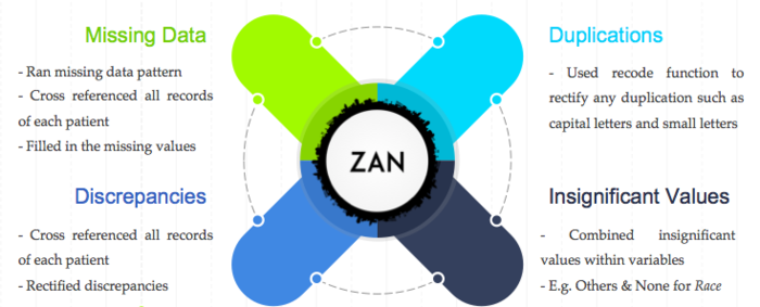
The data had 77,205 records initially. The following diagram shows our team's general data cleaning procedures.
New Variables Derived
As mentioned earlier, the given data does not have some variables, such as appointment age, that were highlighted by other research studies. Using Visit Date, we are able to compute the appointment lead time between a patient’s previous scheduled appointment and the next scheduled appointment. In addition, Clinic Switch is derived to study if there is any impact on the no-show rate of patients whose appointments are switched between the two clinics. There are 12,425 records of patients who have attended both clinics at least once.
After the data preparation process, we retained about 82% of the original data with 63,511 records left.
With two different clinics situated at different parts of Singapore, we realized that there are potential insights that could be gained by heading towards the geospatial direction. It adds two additional factors, location of the clinic and residence of patients into the analysis. Maps also make it easier for us to recognize patterns that were previously buried in rows and columns.
As the data only contains the postal districts and postal codes of the patients, we will need to derive the longitude and latitude points of each postal code. Other issues that arise were some patients have multiple postal codes as they have changed their residence over time and there were 2,503 records showing invalid postal district (denoted by 99).
We cross-referenced patient records and managed to reduce the number of records showing invalid postal district to 216 records. We also updated the records to ensure that each patient will only have one postal code and postal district. With the advice of our project supervisor, we used Tableau 10 to generate the longitude and latitude points.
With the longitude and latitude points, we can also derive the distances of patient’s residence to each clinic. Firstly, we need to convert the coordinates from World Geodetic System, WGS 84 to Singapore Coordinate System, SVY21 before using the below formula to compute the distances.
Postal District Analysis
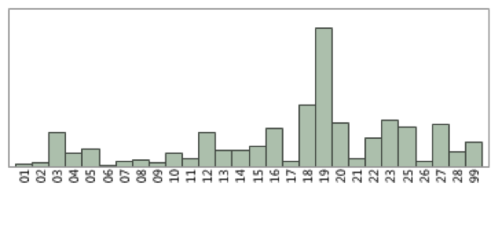
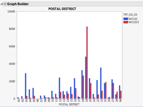
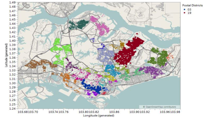
The postal district showed that the main bulk of the patients, in the dataset, resided in District 19. District 19 consists of general location around Serangoon Garden, Hougang and Punggol. Clinic B has a significant number of patients from District 19 due to the close proximity of its location. The below chart depicts the distribution of patients living in each postal district around Singapore. The most densed district (highlighted in red) is District 19.
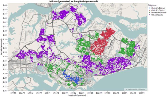
To understand the distribution of patients, we grouped the postal districts into the districts that the clinics are located in, the next immediate districts and other districts. As seen in Figure 9, Clinic A is located in district 3 (highlighted in blue) while clinic B is located in district 19 (highlighted in red). Districts 1, 2, 4, 5, 6, 9, 10, 13, 18, 20 and 28 (highlighted in green) are the immediate neighbours around the respective clinic’s district. The other districts are highlighted in purple. As seen in chart 8, there is high density of patients living in Clinic B’s district.
For modelling, we can either analyze the data of individual records as an isolated episode or analyze the data combined across the patients (grouped data by patient analysis). According to Cohen, Sanborn and Shiffrin (2008), grouping can distort the form of data, and different individuals might perform the task using different processes and parameters. However, they have shown that there are occasions where grouped analysis outperforms individual analysis. To test this literature review, we will use two sandboxes; one for analyzing each individual records and another for analyzing records grouped by patients.
The sandbox for analyzing each individual record can then be segregated further into appointments to see a doctor and appointments to see an allied health professional. The reason being is that the response variable for allied health professionals has an additional category ‘cancelled appointments’. Thus, we have prepared the following for our subsequent models:
- Per episode for doctors (0-Attended, 1-Defaulted): Logistic regression and decision tree
- Per episode for allied health professionals (0-Attended, 1-Cancelled, 2-Defaulted): Multinomial regression and decision tree
- Per patients (0-Attended, 1-Cancelled, 2-Defaulted): Multiple linear regression
As the dependent variable, Plan IND is nominal (contains multiple categorical classes), logistic regression is selected as an appropriate modeling technique to be used. Logistic regression deals with categorical response variable by using a logarithmic transformation on the response variable which allows us to model a nonlinear association in a linear way. It is important to note that logistic regressions work with odds rather than proportion. The odds are simply the ratio of the proportions for the two possible outcomes. If y is the proportion for one outcome, then 1 – y is the proportion for the second outcome.
Dealing with Multicollinearity
As most of the data are categorical variables, we ran chi-square tests to evaluate the relationship of each variable and the dependent variable, Plan IND. This is important as logistic regression is sensitive to extremely high correlation among independent variables, which would give rise to a large standard error parameter estimates. A p-value ≤ 0.05 (as seen in Figure 6) shows that the independent variable is statistically different from the dependent variable. The chi-square tests have shown that there is at least a statistically significant relationship between each variable and the dependent variable.
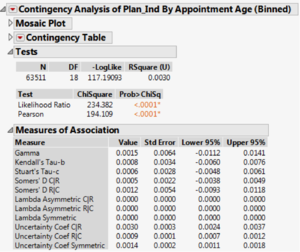
Figure 8: Example of a Chi-Square Test for Plan IND by Appointment Age
Dealing with Complete or Complete-Quasi Separation
When running logistic regression, we may run into a problem of a complete separation or quasi-complete separation. It occurs when a predictor variable is able to predict the response variable perfectly. E.g. Observations with Y= 0 when all values of A1<=2 and observations with Y=1 when A2 have values>2. In such cases, Y separates A completely and there is no need for estimating a model as the maximum likelihood estimate for A1 or A2 does not exist. Thus, we need to make sure that the outcome variable is not a dichotomous version of a variable in the model.
Decision tree modelling is a multiple variable analysis that predicts future observations based on a set of decision rules that recursively splits independent variables into homogeneous zones. It provides unique capabilities to supplement and complement the logistic regression. Unlike logistic regression, decision tree is able to handle incomplete data and does not require any statistical assumptions concerning the data. This is prevalent in the project as some of the patients’ postal codes are missing or invalid to compute any distance from the clinic.
End of excerpt from the Final Conference Paper. For more information on the complete analysis, please download the paper or contact the team.
• Allaeddini, A., Yang, K., Reddy, C. & Yu, S. (2011, February). A Probabilistic Model for Predicting The Probability of No-Shows in Hospital Appointments.
• Cohen. A. L., Sanborn. A. N., Shiffrin. R. M., (2008). Model Evaluation Using Grouped or Individual Data.
• Clark. W. A. V., Avery. K. L. (1975, October). The Effects of Data Aggregation in Statistical Analysis
• Daggy, J., Lawley, M., Willis, D., Thayer, D., Suelzer, C., DeLaurentis, P. C., ... & Sands, L. (2010). Using no-show modeling to improve clinic performance. Health Informatics Journal, 16(4), 246-259.
• Huang, Y., & Hanauer, D.A. (2014, September). Patient No-Show Predictive Model Development using Multiple Data Sources for an Effective Overbooking Approach.
• Ma. N. L., Seemanta. K., Wu. D., Ng. S. S. Y. (2014). Predictive Analytics for Outpatient Appointments.
• Michelle. K. (2011, January). When Absence Speaks Louder than Words: An Object Relational Perspective on No-Show Appointments.
• Michael. L. D., Rachel. M. G., Jerrold. H. M., Robert. J. M., Keri. L. R., Youxu. C. T., Dominic. L. V., (2016, February). Large-Scale No-Show Patterns and Distributions for Clinic Operational Research.
• Molfenter. T. (2013). Reducing Appointment No-Shows: Going From Theory to Practice.
• Muthuraman, K., & Lawley, M. (2008). A stochastic overbooking model for outpatient clinical scheduling with no-shows. Iie Transactions, 40(9), 820-837.
• Naomi. L. L, Audrey P, Matthew. D. R., Bruce. L. (2004). Why We Don’t Come: Patient Perceptions on No-Shows.
• William. S. M, M.S.W., BCD (2001). Why They Don’t Come Back: A Clinical Perspective on The No-Show Client.
• Woo. BS., Ng. TP., Fung. DS., Chan. YH., Lee.YP., Koh. JB., Cai. Y. (2007). Emotional and Behaviorual Problems in Singaporean Children Based on Parent, Teacher and Child Reports.
