AY1516 T2 Team Hew - Prediction

Home

Team

Overview

Project Management

Analysis

Exploratory Analysis (Interim)

Prediction

Claim Amount Distribution Fitting

Analyze Distribution

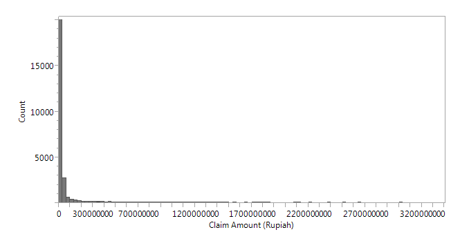
Vaughn and a number of actuaries have mentioned that Claim amounts have to factor in inflation for greater accuracy. However, as the highest inflation rate attained by Indonesia for the time period of study is about 7%, this is rather negligible. Using JMP Pro 12, we first excluded rows where Claim amount = 0 and derived the distribution statistics of:

N	Min	Max	Median	Mean	Standard Deviation
49,066	2,570	3,295,056,701	4,297,418	21,090,896	90,927,485

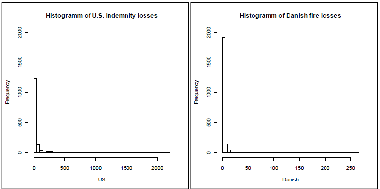
From figure above, we can see that there are many instances of small claim amounts, with few instances of extreme values, and the distribution shape is right skewed. Similar distribution shapes for Claim amounts have also been derived from insurance companies based in other regions, as seen in figure below taken from Eling's Research.

Fit Distribution

We then attempt to fit several distributions on the Claim amounts column, using JMP Pro’s Fit Distribution function. The most suitable distribution selected will be the one which minimizes the -2Log(Likelihood), taken to be a measure of variation or uncertainty in the sample.

We can see that -2Log(Likelihood) is minimized with the LogNormal distribution. According to JMP Pro documentation, maximum likelihood estimation is used in determining the parameters for the LogNormal distribution. Naturally, we can see why the LogNormal distribution derives the lowest -2Log(Likelihood) as the problem of maximizing the likelihood function is reformulated to become a minimization of the negative of the natural logarithm of the likelihood function.

We did another Goodness-of-Fit test using Kolmogrov’s D test with the null hypothesis as “H0: The data is from the LogNormal Distribution”, thus obtaining a D-statistic of 0.048569 and a p-value of 0.01. As p-values are the probability of getting an even more extreme statistic given the true value being tested is at the hypothesized value (usually at zero), a small p-value means that the statistic is unlikely to be that extreme by coincidence. In this case, the p-value of 0.01 is fairly small, indicating significance that the fitted distribution is LogNormal.

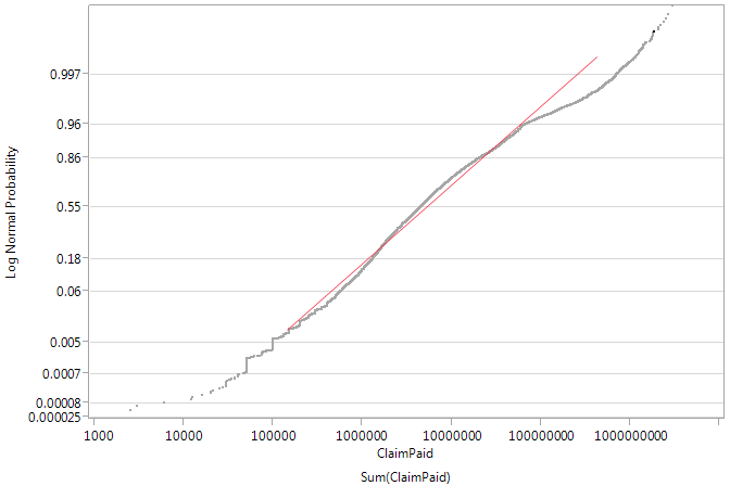
Using JMP Pro’s Diagnostic Plot function, we can visually affirm the goodness-of-fit, as seen in the figure below. The actual Claim amount is plotted against its corresponding estimated LogNormal probability on the Y-axis. We can see that most of the data points fall on the Line of Fit (red line) for Claim amounts within the mid-range, thus depicting a good fit.

Several other papers have adopted to fit Claim amounts with the LogNormal distribution because of its right-skewed shape, and this is in line with our findings. We therefore fit a LogNormal distribution to the Claim amounts, which allows us to use it for prediction or modelling purposes.

Segmentation

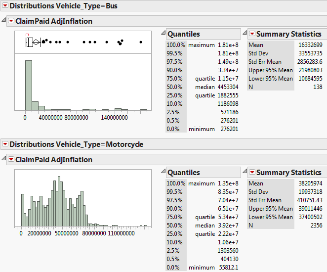
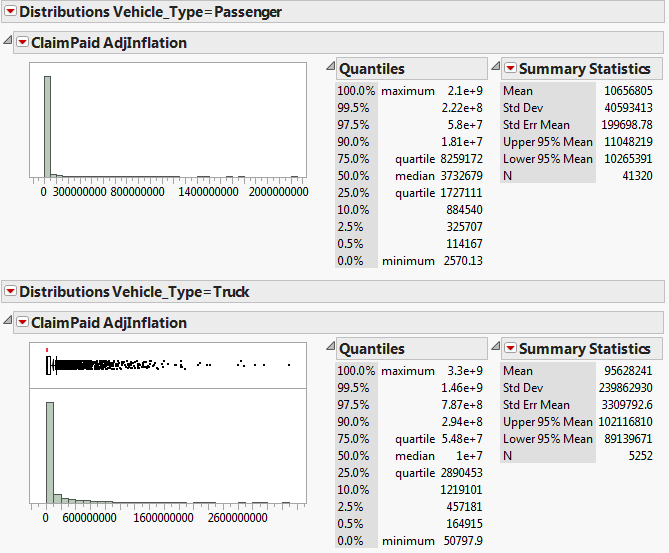
We hypothesized that there would be differences in claim amounts for different vehicle types, due to the varying costs of each vehicle, so we proceeded to segment the dataset by the Vehicle Type (Passenger Car, Bus, Truck, Motorcycle) and plot the Claim amount distributions for each segment:

We can see that the distribution shape for Motorcycles is different as compared to the other Vehicle Types, as about 90% of the claims were theft-related. The other Vehicle Types have a similar right-skewed distribution which we can fit a LogNormal distribution, albeit with different parameter values due to the differences in Claim amounts. Claim amount is generally higher for larger Vehicle Types.

Multiple Linear Regression

Applying Log Transformation

We first attempted a prediction of Claim amounts on the Passenger Car Segment of the dataset. A natural logarithm transformation was applied to normalize the Claim amounts as shown below:

Initial Distribution	After Applying Log Transformation

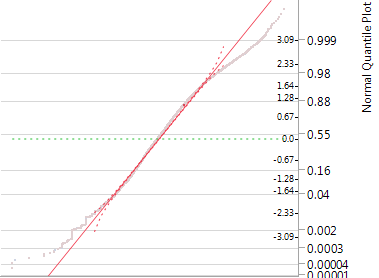
We can see that the Mean of 15.0673 is now approximately equal to the Median of 15.0318, indicating a Normal distribution. This is further confirmed by the Normal Quantile plot below which shows that the data points are close to the line of best fit:

Multiple Linear Regression

We then set out to predict the Log(Claim amount) of the Passenger Car segment, using the following independent variables listed below. Our approach was to first include all possible variables that were useful in the predictive model, then analyze the results to remove the insignificant variables and improve model accuracy.

Variable	Values	Description
VehAge_Current	Continuous Numerical	Current Vehicle Age
Bus_Ind	New Business / Renewal Business	Business Indicator
Driver_Age	Continuous Numerical	Only recorded when a claim is made
Corppers	Corporate / Personal	Account Type
At_Fault	At Fault / Not At Fault	Whether the Claimant caused the accident that resulted in the claim
Veh_Make	Audi / BMW / Chevrolet / Chrysler / Daihatsu / Ford / Honda / Hyundai / Isuzu / Jaguar / Land rover / Mazda / Mercedes Benz/ Mitsubishi / Nissan / Opel / Peugeot / Proton / Subaru / Suzuki / Timor / Toyota / Volkswagen	Vehicle Brand
Log(SumInsured)	Continuous Numerical	Natural Logarithm Transformation of the vehicle's Sum Insured amount
Coverage_period	Categorical Numerical	Policy coverage period in years
Jap_Ind	Japanese / Local	Japanese Customer Indicator
Cover Type	Comprehensive / Total Loss Order	Policy Coverage Type
Channel	Agent / Bank / Broker / Coinsurance / Dealer / Direct / Leasing	Sales Channel
Cause_Type	Collision / Fire / Flood / Grazed (humans) / Grazed (non-vehicle) / Grazed (vehicle) / Impact (humans) / Impact (non-vehicle) / Impact (vehicle) / Others	Cause of the claim

Splitting the dataset by a mix of 60% (Training Set), 20% (Validation Set), 20% (Test Set), the following results were obtained:

	Training Set	Validation Set	Test Set
R-Square	0.288	0.274	0.223

Even with all the possible variables used as predictors, the R-Square stands at a low value of 0.288. The same approach was taken on other predictive methods like Decision Trees and Neural Networks, but yielded a similar low R-Square value of between 0.3-0.4 thus highlighting the dataset's lack of predictive ability.

Recommendations

Suggested improvements to dataset:

• The Bus_Ind variable allows us to see which policy is a renewal, however, it does not tell us which particular customer has made a renewal, as individual customer names are not recorded, but rather, the Leasing Agent names are recorded. Having the actual customer names in the dataset can open up many possibilities for Predictive Analytics - e.g. to identify hidden customer segments/clusters and also to predict customer churn rate.
• This can be supplemented with further customer demographic data like the age, gender, income level, address, etc.
• Record claim cause in the form of an additional accident report instead of just classifying it in categories. This can allow for text mining to be applied in conjunction with other predictive methods to detect fraud.

References

- ↑ Vaughn, Trent R. (1996), Simulation Models for Self-Insurance
- ↑ Eling, M. (2011), Fitting Insurance Claims to Skewed Distributions, Working Papers on Risk Management and Insurance, No. 98, November 2011
- ↑ Adeleke, Ismail A., Ibiwoye, A. (2011), Modelling claim sizes in Personal Line non-life insurance, International Business & Economics Research Journal - February 2011, Vol. 10, No. 2, pp. 21-38