ANLY482 AY2016-17 T2 Group11: Project Findings Final

Return to ANLY482 AY2016-17 Home Page

Interim

Final

Paper 1 Final Slides | Final Practice Research Paper 1 | Paper 1 Poster
Paper 2 Final Slides | Final Practice Research Paper 2 | Paper 2 Poster
Paper 3 Final Slides | Final Practice Research Paper 3 | Paper 3 Poster

Paper 1: Using Latent Class Analysis to Standardise Scores from the PISA Global Education Survey to Determine Differences between Schools in Singapore

Singapore’s Ministry of Education started a slogan, “every school a good school” in 2013. However, the public sentiment is that all students do not start on an equal footing.

OECD education director Andreas Schleicher mentioned that “Singapore managed to achieve excellence without wide differences between children from wealthy and disadvantaged families.

This begs the following questions: Is it fair to state that all schools are good schools?

Objective

Through our analysis, we seek to determine if there are differences between schools in Singapore based on their PISA performance .

Methodology

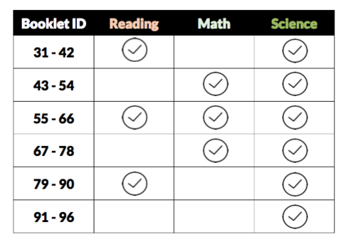
From the 2015 PISA data, there were 66 booklets use and each booklet contained different number of questions and a combination of science questions together with reading and/or math questions.

Latent class analysis (LCA) will be used to classify questions to their most likely latent classes (easy, medium, or hard).

Each question’s weight will be adjusted based on the LCA results to determine the standardized score of each student.

Literature Review

Latent Class Analysis

Latent class analysis (LCA) is a statistical method for finding subtypes of related cases (latent classes) from multivariate categorical data. The results of LCA can be used to classify cases to their most likely latent classes. Common areas for the use of LCA are in health research, marketing research, sociology, psychology, and education. This clustering algorithm offers several advantages over traditional clustering approaches such as K-means such as assigning a probability to the cluster membership for each data point instead of relying on the distances to biased cluster means and LCA provides various diagnostic information such as common statistics, Bayesian information criterion (BIC), and p-value to determine the number of clusters and the significance of the variables’ effects.

This method was applied on the 2012 PISA data of Taiwan to objectively classify students’ learning strategies to determine the optimal fitting latent class model of students’ performance on a learning strategy assessment and to explore the mathematical literacy of students who used various learning strategies. The findings of the research shows that a four class model was the optimal fit model of learning strategy based on the BIC and adjusted BIC when comparing the four class model to other models of two to five classes. The study showed that Taiwanese students who were classified under the “multiple strategies” and “elaboration and control strategies” group (multiple learning strategy) tend to score higher than average while students classified under the “memorization” and “control” group (single learning strategy) performed lower than average.

Data Preparation

From the PISA 2015 Database, we only used the files relevant for the project which are the student questionnaire data, school questionnaire data, and cognitive item data. The other files which were not relevant for us were the teacher questionnaire data and the questionnaire timing data. We also used the codebook data file for easy reference.

Upon initial exploration of the cognitive item data, which contains information on how students answered mathematics, reading, and science questions, we noticed that there were multiple booklets used and discovered a pattern. Booklets 31 to 96 were used for schools in Singapore and all booklets contained questions for Science together with Reading and/or Mathematics questions or just purely Science questions. Each booklet contained various number of questions and thus the total scores of each student cannot be compared across booklets. LCA will be used to determine the difficulty of the each question based on how well the students performed for the question and then the questions will be adjusted based on the difficulty.

Filtering to Singapore Data

From the raw files extracted from the PISA 2015 database, we only kept those with the 3 character country code of “SGP” as we only want the data related to Singapore. This is applied to the student questionnaire data, teacher questionnaire data and cognitive item data. This provided us with 6115 students and 177 schools of which 168 are public schools while the other 9 are private schools.

Removed columns with no response or same value in all entries

The next step was to remove columns with no responses from all schools and students. Columns that contained the same value in all entries were also removed such as Region and OECD Country. For the student questionnaire data and teacher questionnaire data, this is the last step for data preparation while more steps are needed for the cognitive item data in terms of having a standardized score for each student.

Kept scored and coded responses from cognitive data

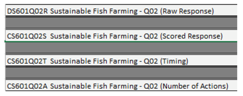
In the cognitive item data, each question contained several information such as raw response, scored response, timing, and number of actions. The only columns which were kept for the cognitive item data were the scored responses or coded responses as this contains the information on whether the student received any points for the question.

Adjust Scores

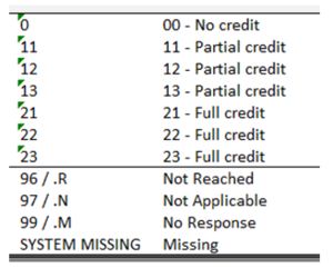
Questions in the cognitive item data were scored differently as some questions were given the value of 1 for partial credit and 2 for full credit. We decided to allocate 0 for no credit, 0.5 for partial credit, and 1 for full credit. For missing values, the value of 9999 was given.

Transposed Questions

In Excel, each student belonged to a row and the columns contained the student’s score for the questions that were answered. We then transposed the questions from columns to rows in JMP Pro to get the count and distribution of scoring classification for each question.

As there were different booklets used, each student only answered a small portion of all the questions that were available. When the cognitive item data was transposed into JMP Pro, the questions which were not in the booklet answered by the students were also included and this gave a total of 2,109,675 rows. After removing rows which did not contain any value in N(0), N(0.5), N(1), and N(9999), we were left with 314,366 rows.

Bin Scoring Classifications

We then proceeded to bin the scoring classifications based on its distribution for every question. 10 bins were used of 10% ranges. The data is then ready for LCA after this step.

Data Analysis

Latent Class Analysis

With the binned scoring classifications, latent class analysis can be performed to determine the most likely difficulty of the questions. To determine the number of clusters to be used, a selection of 2 to 5 clusters was chosen to determine the best fit to the data. The Bayesian information criteria (BIC) was looked at in order to determine the best model fit.

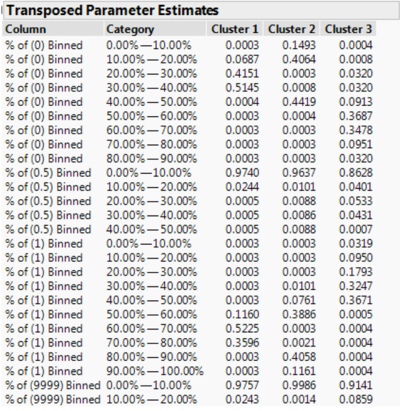
From the results, the Bayesian information criteria (BIC) was looked at for two to five clusters and the lowest value was determined to be the model with the best fit. From table 1, we could see that the latent class analysis with 4 clusters provided the best fit with a BIC value of 2921.4. However, the latent class analysis with 3 clusters also provided a low BIC value of 2927.15 and thus, we decided to use the latent class analysis with 3 clusters to signify the 3 difficulties for the questions which are easy, medium, and hard.

Discussion on LCA Results

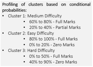
From the transposed parameter estimates, the probability of each question’s most likely difficulty can be determined based on the conditional probabilities of each cluster. From cluster 1, we can see that the biggest contributor comes from 60.00% to 80.00% of % of (1) Binned which are questions where students have gotten full marks and the second biggest contributor comes from 20.00% to 40.00% of % of (0) Binned which are questions where students have gotten no marks. From the contributors we can profile this cluster to be questions which have medium difficulty. For cluster 2, the biggest contributor comes from 80.00% to 100.00% of % of (1) Binned and 0.00% to 20.00% of % of (0) Binned which means these are questions where students generally get full marks and thus we can profile this cluster to be questions which have easy difficulty. For cluster 3, the biggest contributors are 0.00% to 50.00% of % of (1) Binned, 40.00% to 90.00% of % of (0) Binned, and 10.00% to 40.00% of % of (0.5) Binned. We can profile this cluster to be questions which have hard difficulty since these are questions where more students get no marks or only partial marks.

Standardized Scoring

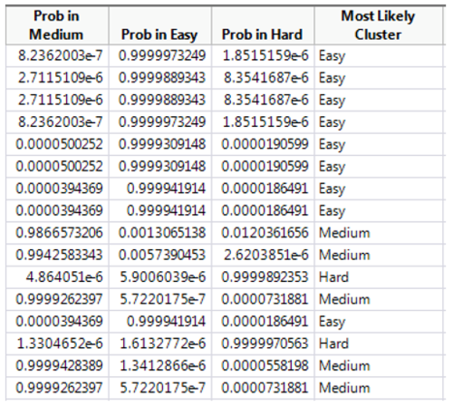
From the latent class analysis, 3 columns are created in the data table with the binned scoring classifications which are the probability of each difficulty (easy, medium, and hard). From these 3 columns, the most likely cluster is derived based on the column with the highest probability.

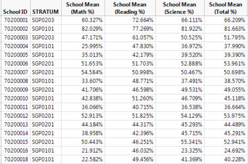
Each question’s weight is then adjusted based on the difficulty of the question and the total score for each student can then be computed for. With the adjusted total score for every student, each school’s performance can be calculated for based on the scores of the students.

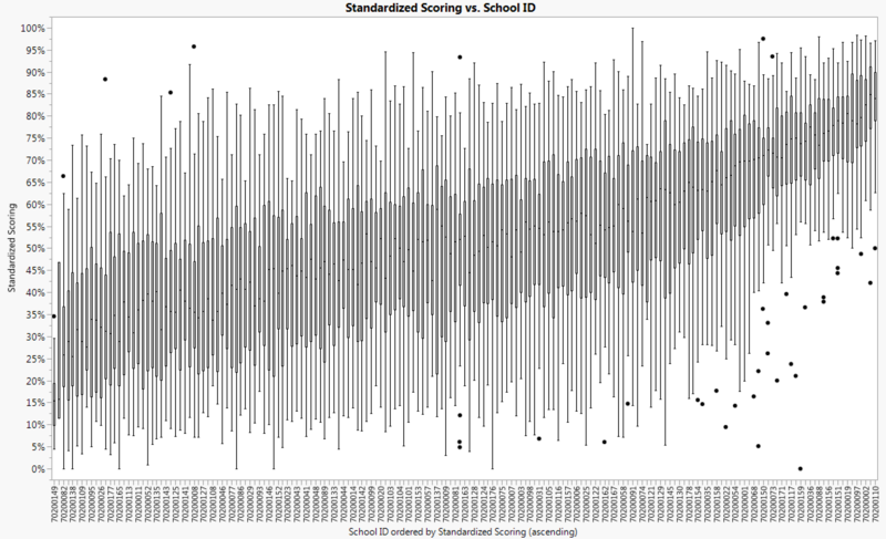
Looking at the boxplot of the scores of all schools, we see how schools in Singapore are different in terms of their performance. There are schools which perform exceptionally well as seen in the right side of the image below while there are also schools which did not perform well which is contrary to the notion of every school being a good school. Another point to highlight in the box plot is the number of outliers for schools which performed well. Although majority of the students in the high performing schools did well, there are a lot more outliers compared to schools in the middle and bottom tier.

Conclusion

Through latent class analysis, questions were placed in clusters and these clusters were profiled based on the parameter estimates to determine the associated difficulty of the cluster (easy, medium, or hard). Each question’s weight was then adjusted to get the standardized score of every student for comparison. Through the analysis, there is indeed a difference between schools in Singapore based on their performance in the 2015 PISA global education survey.

Paper 2: An Analysis of Singapore School Performance in the Programme for International Student Assessment (PISA) Global Education Survey

Singapore’s Ministry of Education started a slogan, “every school a good school” in 2013. However, the public sentiment is that all students do not start on an equal footing.

This begs the following questions: What determines the differences in results across schools in Singapore? Should more support can and should be given to students from less privileged backgrounds?

Objective

Through our analysis, we seek to explore the factors contributing to the differences in overall scores and science scores across all schools.

Methodology

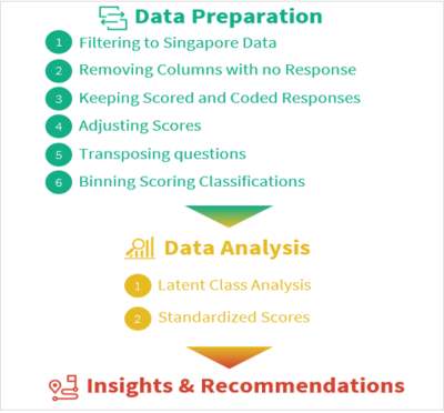
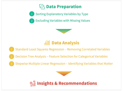
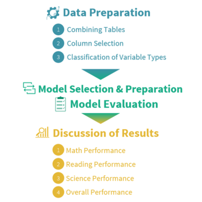
The image above illustrates the analytical process used for this paper. After data preparation, we proceeded with the data analysis using several analytical techniques – since the dataset contains both continuous and categorical explanatory variables, there is a need to separate the two types of explanatory variables during the initial feature selection, prior to conducting the stepwise regression model. For the continuous explanatory variables, we used the standard least squares regression method to remove correlated variables. For the categorical explanatory variables, we will be using decision tree for feature selection. Next, the team conducted multiple linear regression to identify and analyze the factors that affect the scores of the schools, using the observations from the data analysis segment to provide key insights and recommendations.

A regression model is a mathematical model that explains and predicts a continuous response variable. For our analysis, a regression model will be developed to explain why certain schools score better than others. Multiple linear regression is the key technique selected to derive our insights due to its flexibility in allowing us to use both continuous and categorical variables. In this case, the explanatory variables are derived from the questions posted to the school, and the response variables are the schools’ mean overall score and schools’ mean science score, which will be analyzed separately.

Literature Review

Multiple Linear Regression

There has been numerous research done across the world using the PISA results, which is released once every three years. Most of the research are done at an international level, and while there are country-specific research, there are minimal research done on Singapore’s results. Therefore, we are interested in analyzing Singapore’s results to find out if there are similarities and differences.

There are multiple findings stating that a student’s performance is generally better when their socioeconomic status is higher, and socioeconomically advantaged students tend to get better scores as compared to their disadvantaged peers regardless of countries and economies. Naturally, drawing it back to the comparison schools’ performance, it can be hypothesized that schools with greater percentage of disadvantaged students from a socioeconomic perspective tend to perform more poorly overall.

We decided to use multiple linear regression as the main technique to determine the correlations between the mean school overall or science score and the questions in the school questionnaire filled in by the principal or relevant school personnel. Past research has also used the regression model to analyze and even predict how well students will do for a specific subject such as Mathematics. Rather than a predictive model, we intend to create an explanatory model to analyze variables affecting schools’ performance.

Data Preparation

Sorting Variables by Type

Using the codebook provided by OECD, the team sorted the questions from the school questionnaire into continuous, ordinal or nominal variables by observing the question types.

Excluding variables with missing values

Response Variables: School ID 29 was removed due to missing values for majority of the questions

Explanatory Variables: Arbitrary threshold created – no more than 20%, or 35.4 out of 177 missing data points should exist. Based on the threshold, we excluded one question, “SC014Q01NA”.

Data Analysis

Standard Least Squares Regression – Removing Correlated Variables

For the remaining continuous explanatory variables, we conducted standard least squares regression to identify and exclude correlated variables through observing the correlation of estimates, ensuring that they do not exceed a threshold of +/- 0.7.

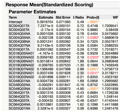
The variables were removed conservatively, as we aim to retain as many variables as possible, in order to avoid missing out on variables that might have a huge effect on the response variable. Three iterations of standard least squares regression were done to ensure that no remaining variables were correlated. This was further confirmed by checking the Variance Inflation Factors (VIF), as shown in the figure below. VIF is useful in determining multicollinearity within variables. While there are no formal criteria with regard to an acceptable level of VIF, a common recommendation is a value of ten; and a clear signal of multicollinearity is when VIF is greater than eight. However, it is also important to pay attention to variables that have a VIF of five or more. In this case, the final set of selected variables have VIF values of less than five, indicating that multicollinearity does not exist in the final iteration of our standard least squares regression model.

After three iterations of standard least squares regression for both response variables, there was a final number of 22 continuous explanatory variables for schools’ mean overall scores, and 21 continuous explanatory variables for schools’ mean science scores. These variables will be used for the final step, stepwise regression.

Decision Tree Analysis – Feature Selection

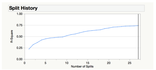
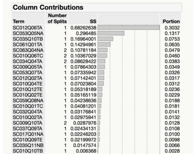
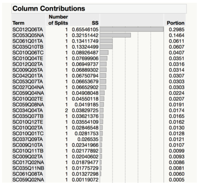
Due to the excessive number of categorical explanatory variables, instead of including all of them in the stepwise multiple linear regression model, we used decision tree to conduct feature selection, whereby the variables which are important and affect the response variables will be selected for stepwise regression. The number of splits is determined by ensuring that for each split conducted, the R-square value continues to rise and does not reach a plateau by observing the split history graph as seen in the figure below. In our case, it reached saturation prior to the graph reaching a plateau.

The selection of variables is determined by the logworth of the variable, whereby all variables with positive logworth (greater than zero) will be selected, as seen in the figures below.

Stepwise Multiple Linear Regression – Identifying Variables that Matter

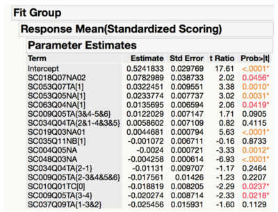
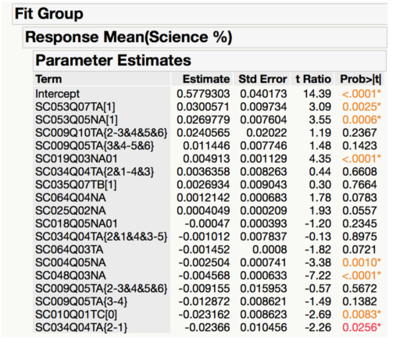
After the above feature selection processes, 22 continuous variables and 23 categorical variables were used for the regression model for the mean school overall scores, while 21 continuous variables and 27 categorical variables were used for the mean school science scores. Backward, forward and mixed stepwise regression models were generated, where a selection criteria for a variable to enter or leave was if they had a p-value of less than 0.05 for both schools’ mean overall score and schools’ mean science score.

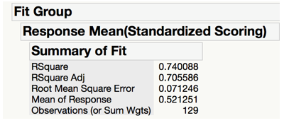
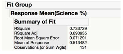
Upon comparison of the three methods, backward stepwise regression results in the highest adjusted R-square for both mean school overall scores (adjusted R-square of 0.7056) and mean school science scores (adjusted R-square of 0.6909), as seen in the figures above. In other words, the set of explanatory variables highlighted by the backward stepwise regression can account for 70.56% of the variation in the mean school overall scores, and the explanatory variables highlighted by the backward stepwise regression explains 69.09% of the variation in the mean school science scores. Given that the variables derived from the backward stepwise regression model allows us to best explain the variation in the schools’ performance, the results from backward stepwise regression will be used for the analysis.

Insights from Stepwise Regression Model

Variables Affecting Overall Score

Parents involvement in school decisions (SC063Q04NA)

It is recommended that schools include parents in their decision-making process for school-related issues, as schools that have chosen to include parents have fared better at the PISA results.

This is in line with recent trends where schools aim to engage parents beyond the “superficial” purposes such as fundraising or attending events. One potential reason for this variable to be significant to the schools’ mean overall scores is that parents feel more ownership when they get to participate in school decisions, encouraging them to contribute their valuable knowledge, skills and viewpoints.

Education level of part-time teachers (SC018Q07NA02)

Another interesting insight is that having a greater number of part-time teachers with a degree from a second stage of tertiary education, such as masters or doctoral degree, results in better overall scores.

Variables Affecting Science Scores

Participation in professional development programmes for teachers (SC025Q02NA)

It is comforting to note that having greater number of science teachers attending professional development programmes contribute to better school scores, as it shows that these programmes are effective in preparing the teachers to become better educators, allowing the students to learn more effectively.

Proportion of parents’ participation in school-related activities (SC064Q04NA)

Similar to the previous finding for overall scores where parents’ participation contributes to better school results (overall scores), the greater the proportion of parents participating in school-related activities such as volunteering, the better the school’s performance in science.

Frequency of principal’s engagement with teachers to create a school culture of continuous improvement (SC009Q10TA)

Intriguingly, there is an ideal frequency for principals to engage their teachers to create a school culture of continuous improvement, which is “1-2 times during the year”. This shows that it is important for principals or leaders to remind teachers of the need to continuously improve, and that status quo is never good enough. However, at the same time, it is critical to not do it too often, as it may potentially divert too much time and effort from other important matters such as time spent on the curriculum or teaching methods.

Variables Affecting Both Overall Scores And Science Scores

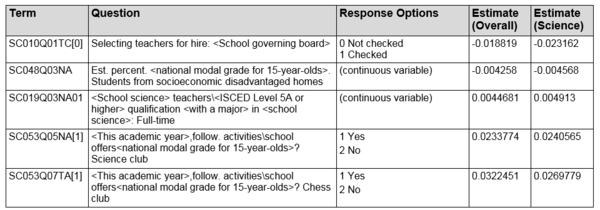
There are 11 variables affecting both the schools’ mean overall score and schools’ mean science score relatively significantly, and five of them are displayed in the table below.

Significance of extra-curricular activities (SC053Q05NA & SC053Q07TA)

As illustrated in the table above, schools that offer extra-curricular activities, specifically Science Club and Chess Club tend to do better. These variables are also two of the variables with the highest absolute parameter estimate values, indicating that they have a relatively more significant effect on the mean schools’ scores. Therefore, the presence of these extra-curricular activities clubs is a good determinant of the school’s capabilities, potentially due to the fact that these clubs enrich the students’ learning and growth through activities that engage their minds effectively.

Percentage of students from socioeconomic disadvantaged homes (SC048Q03NA)

Schools with a higher percentage of students from socioeconomic disadvantaged homes tend to do less well in the PISA survey. This is in line with past research, which has shown that socio-economic status does affect a student’s performance, whereby “home background makes a substantial contribution to student differences”. This further illustrates the need for relevant stakeholders such as the government, more specifically the Ministry of Education, to ensure that students from socioeconomic disadvantaged homes are given sufficient support to start on an equal footing, and to be given the chance to reach their full potential despite coming from a less privileged background. In the context of schools, this can be done by identifying schools with higher percentage of socioeconomic disadvantage families, and providing more subsidies or grants for free tuition or enrichment courses. This is especially the case in Singapore, where more than 60% of parents of secondary school children, the target age group for this survey, send their children for tuition.

Role of school governing board in selection of teachers for hire

Interestingly, the school governing board should ideally play a part in selecting teachers for hire, since schools that did not include the school governing board in the selection process tend to do worse. This may be due to the lower level of structure or lower standards in the selection process for hiring teachers if the school governing board was not involved. Another potential reason is the lack of experience within the hiring panel if the school governing board were to be left out of the process.

Education level of full-time science teachers (SC019Q03NA01)

Schools with a greater number of full-time school science teachers with minimally a bachelor’s degree tend to do better. As expected, this variable has a greater impact on the schools’ mean science scores compared to the overall scores. This implies that education level of the teachers do affect their students’ performance, likely due to the way they teach or conduct lessons, given that the content of the curriculum is held constant. Therefore, schools that wish to see better academic results can consider investing in hiring more teachers with a bachelor’s degree.

Conclusion

Given that one of the contributing variables affecting school performance is the percentage of students from socioeconomic disadvantaged backgrounds, it is a telltale sign that there is indeed a difference across schools with regard to their starting ground. Therefore, to ensure that all schools can provide the same support to their students, the Ministry of Education (MOE), as well as the schools themselves, can consider our recommendations in the following three broad areas:

1. Training and Development for teachers
2. Fine-tuning the selection process for hiring teachers
3. Increasing parents’ involvement through meaningful engagement

For training and development, the school can focus on professional development courses aimed at improving improve the overall quality of teaching across all teaching staff. Schools should not have to decide on budget allocation between supporting students with less privileged background and training programmes for teachers. Ideally, MOE should aim to provide more grants to schools with a greater percentage of less privileged students, with the specific purpose of ensuring that the students from socioeconomic disadvantaged backgrounds get the support they need, be it in terms of having a wholesome meal at school, or attending enrichment courses, which has become a norm in Singapore. With regard to the selection process for hiring teachers, MOE can consider allocating the talent pool of teachers with tertiary education equally across all schools. Furthermore, from the results, it can be seen that the school governing body should play a role in the selection process of teachers as well. Finally, parents’ involvement in school activities should be encouraged as it increases the parents’ sense of ownership in their children’s education journey, allowing them to feel more invested and hence dedicate more effort and time to guiding and educating their child academically.

Paper 3: Using Partition Models to Identify Key Differences Between Top Performing and Poor Performing Students

Objective

Identifying key characteristic differences between Top performing students and the Poorer performing students in Math, Reading, Science, and Overall scores in the 2015 PISA test.

Methodology

Literature Review

Decision Tree

Past works using Decision Tree models on Education datasets focuses more on using the models as a predictive tool instead of an explanatory tool. In the work by Priyanka and team, they study various Decision Tree algorithms to evaluate the best one for classifying educational data. Harwait and Amby, used Decision Tree models to determine the characteristics to consider for admission in building a student admission selection model. Mashael and Muna applied Decision Tress to predict student’s final GPA based on student’s grades in previous courses. Quadril and Kalyankar adopted Decision Tree techniques to predict and identify students who are more likely to drop out of school based on past records, and using the predictions as a guide for schools and educators to identify appropriate strategies to prevent the student from dropping out of school. These works offer interesting insights on how Decision Tree models can be used to efficiently on education datasets in model construction for analyzing, explaining, or predicting the data available.

Partition Models

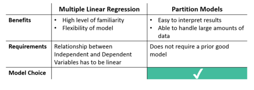
In Partition models, the data is recursively partitioned according to the relationship between the dependent and independent variables to form a decision tree. The benefits of using such models is that the results are easy to interpret, it is able to handle a large amount of data, and does not require a prior good model for us to explore the relationships within the dataset.

Bootstrap Forest

Another type of partition modelling is that of a Bootstrap Forest (Random decision forests), first created by Tin Kam Ho. In this model, many decision trees are built, and subsequently combined to form a more powerful model. It averages the outcome of all the decision trees built to arrive at the final model output. Boosted Tree is another partition model used in our analysis. It is a process of fitting many small decision trees sequentially (layer by layer), to build a large decision tree. As the tree fits layer by layer, it corrects the poor fitting of data from the previous layers, by fitting according to the residuals of previous layers. The final output is the sum of the residuals across all layers.

Data Preparation

Combining Tables

The Standardized Scoring Table, from the scoring standardization performed in Paper 1, and Student Questionnaire Table from the PISA database, both containing 6,115 records, are combined into a single table using left join.

Column Selection

Calculated response columns, such as “PV1SCIE – Plausible Value 1 in Science”, “UNIT - REP_BWGT: RANDOMLY ASSIGNED UNIT NUMBER”, and Warm Likelihood Estimates (WLE) response columns are excluded from our analysis. Only response columns with question terms are kept for our explanatory analysis.

Classification of Variable Types

Referencing the Codebook obtained from the OECD PISA 2015 Database, variables are classified into continuous, nominal, and ordinal types.

Model Selection

When considering an explanatory model for our dataset, we initially considered using both Multiple Linear Regression (MLR) and Partition Models. While performing model fitting using MLR, we notice that the MLR model does not fit well with the dataset used, as there are very few continuous independent variables to draw a meaningful linear relationship with the Standardized Scores of student’s. Since most of the independent variables are categorical in nature, we chose to adopt the recursive tree Partition Models for our explanatory analysis.

Model Preparation

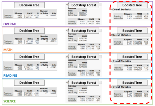
To better understand the differences between top performing students and poor performing ones, we employed the Decision Tree, Bootstrap Forest, and Boosted Tree Partition Methods in JMP Pro 13. A validation factor of 0.3 is used for all three methods. Standardized Scores are assigned to the Response role (Y), and all selected terms from Student Questionnaire are assigned to the Factor role (X). Default options are used for both Bootstrap Forest and Boosted Tree methods.

Model Evaluation

Based on the results shown below, the Boosted Tree is the chosen model for further evaluation, as it generally has a higher Validation RSquared value across the three partitioning models. The difference in RMSE values between Training and Validation sets for the Boosted Tree is also in general, lesser that the other two models, suggesting that the result of the Boosted Tree has less overfitting issues compared to the other two models.

Data Analysis

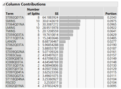
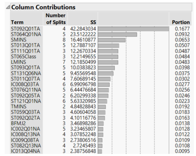
In order to identify factors with strong influence in student’s scores, we only consider Column Contributions with Portion greater than 0.01. Further visualization is performed on selected unique factors for each subjects to discover how the factor influences student’s scores.

Math Performance

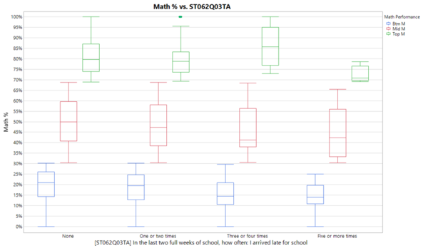
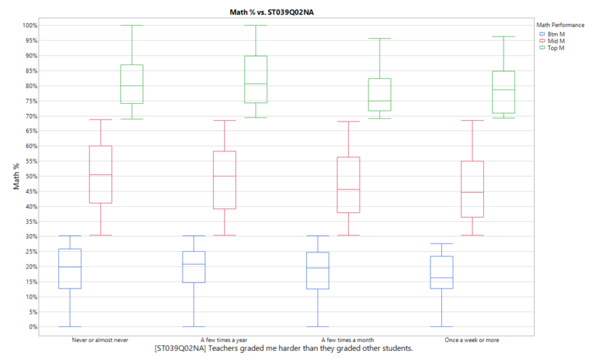
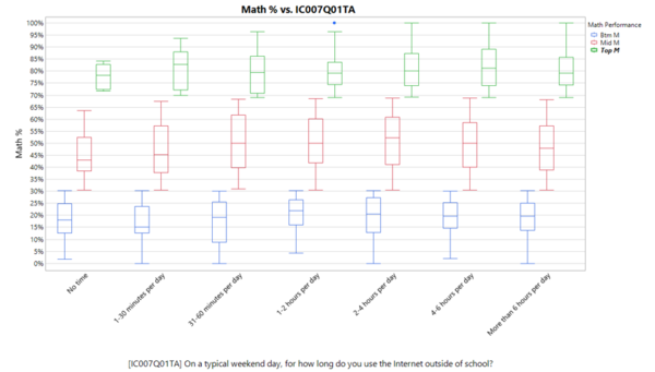
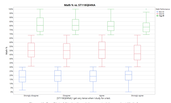
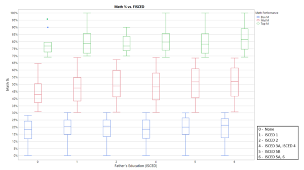
Of the factors having relatively high Column Contributions of above 0.01 for student math scores, we will zoom in on unique factors and their relationship to student’s math performance. Factors which will be discussed further in relation to math performance are student’s punctuality (ST062Q03TA), student’s perception on how they are graded (ST039Q02NA), duration of internet usage over the weekend (IC007Q01TA), how student’s feel when studying for a test (ST118Q04NA), as well as their father’s education level (FISCED).

From the figure below, we can deduce that for students with poorer (Mid and Btm) performance in Math, those who arrive late for at most two times score on average 5% more than students who are late for more than three times. An interesting thing to note is that for top performing Math students, those who arrive late for school for three or four times are observed to score on average 5% better than the more punctual students. Also, students who are late for at least five times in two weeks achieved lower scores in comparison with the rest. Understanding their cause of lateness could be a first step in helping them improve their Math performance.

The figure below shows that for students with math scores in the bottom 25th percentile, those who report that their teachers seem to grade them harder compared to the other students at least once a week or more generally score around 5% lower than students who view their teacher as fairer in grading their work. To reduce students’ perception on how they are graded by their teachers, schools can consider increasing the adoption of technology in grading students’ work.

Surprisingly, as shown in the figure below, students who rarely use internet over the weekend (less than 30 minutes per day) generally score lower compared to their peers who are on the internet for a longer duration. It is observed that students who use the internet for between 30 minutes to 4 hours per day over the weekend perform better in Math. From this observation, parents could consider allowing more internet usage time instead of prohibiting the use of it, while at the same time monitoring what their child is using the internet for, as a preventive measure.

In relation to the figure below, it is interesting to note that amongst the poorer performing students, the more they feel tense when studying for a test, the better they perform. In contrast, for the top performers, the more tense they feel, the poorer their test scores. A possible explanation for this observation could be that students who are good in the subject feel more confident and prepared when studying for a test, whereas students who are weaker in the subject feel less confident and less prepared, thus feel more tense when they are studying for a test.

A general observation from the analysis of a student’s father’s education level in the figure below is that across student performances, the more educated their father is, the better the student performs. This reveals that socioeconomic factors do play an important part in students’ test performance.

Reading Performance

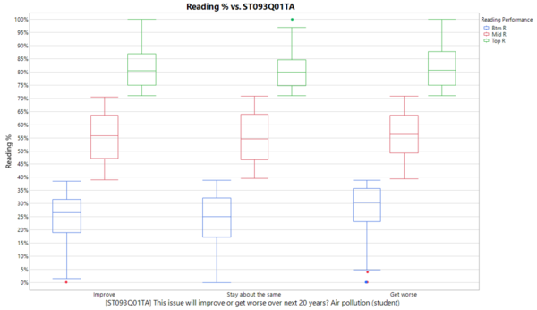
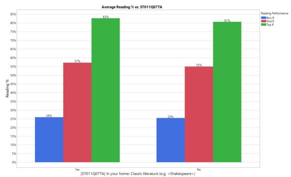
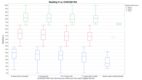
Unique factors for student’s reading scores, such as their perception on environmental issues (ST093Q01TA), availability of classic literature at home (ST011Q07TA), and their age of exposure to digital devices (IC002Q01NA), will be further analyzed to come up with possible explanations on how these factors potentially influence a student’s reading performance score.

Students who perform better in the Reading component amongst their performance groups, as reflected in the figure below, are for the opinion that the air pollution issue would get worse over the next 20 years. A possible explanation for this is that this group of students who are less optimistic of an improvement in the air pollution issue, reads widely and are exposed to the negative reports of air pollution around the world.

Across their performances in the test, students with classic literature at home tend to perform around 2% better than students who do not have classic literature at home, as seen in the figure below. An implication from this observation is that the type and variety of books available at home could have an influence in student’s reading performance in school.

The figure below shows that the younger the students are exposed to digital devices, the better their reading performance. Students who have never used a digital device prior to the test scored significantly lower compared to students in the same performance band. The lack of computer literacy could be the main cause hindering their performance in the test. With more exposure to technology following Singapore’s Smart Nation initiative, this issue would be better tackled, and hopefully in the next PISA assessment, the age of exposure to digital device would not be a key factor influencing student’s test performance.

Science Performance

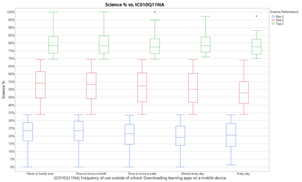
Student’s frequency of downloading learning apps on mobile devices (IC010Q11NA) will be studied further to better understand how the downloading of learning apps influences a student’s science test scores.

In the figure below, students who download learning apps at least once or twice a week are shown to have lower Science scores compared to the less frequent users. This could be due to the differences in syllabus of the learning apps compared to the Science syllabus taught in schools.

Overall Performance

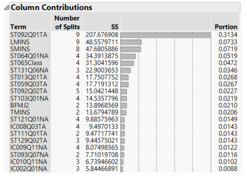
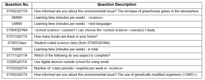
The table below shows all the similar factors across all subjects as well as the overall scores. For our analysis, we will focus on questions pertaining to their general knowledge (ST092Q01TA), amount of time spent studying (TMINS), and the level of education the student expects to complete (ST111Q01TA), in relation to their performance in the test.

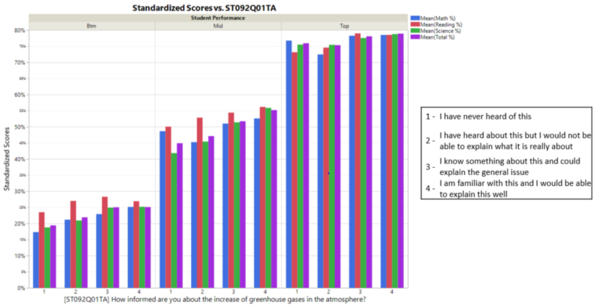
Comparing the similar factors across all subjects, student’s response to their understanding of greenhouse gases has the most effect on their performance. As shown in the figure below, comparing students in the top 25%, middle 50%, and bottom 25% quantiles, students in each group who have better knowledge of greenhouse gases tend to have higher scores.

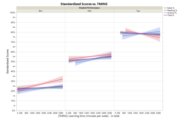
When comparing the learning time spent per week among the top, middle, and bottom performing students, the more time spent learning, the better the test scores for middle and bottom performers. In contrast, as the learning time increases, the lower the test scores of top performing students in Reading and Science, and an upward trend for Math scores. From the figure below, the optimal learning time for top performers is observed to be 1800 minutes per week, around 2500 minutes per week for middle performers, and around 2200 minutes per week for the bottom performers.

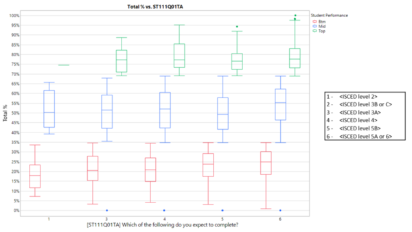
With regards to the aspirational effects on student’s performance, the more aspirational the students are, the better their performance across performance levels, as reflected in the figure below. Students who expect to complete a degree program (6) generally performs on average 3% better than students who expect to complete up to diploma level (5).

Conclusion

In understanding the factors influencing student’s performance in Reading, Mathematics, and Science, we learned that socioeconomic factors, such as the Parent’s education level, availability of digital devices at home, has a positive effect on student’s test scores. In addition, class environment plays a part in the performance of the different groups of students. The perceived fairness of a teacher when grading students’ work is seen to have a positively strong influence in student’s performance. Student’s age of exposure to digital devices is also found to have a strong effect on their test scores, in particular those who have never interacted with digital devices prior to the test performed poorly. In line with the Singapore Government’s Smart Nation Masterplan, an early exposure to technology might improve Singapore’s performance in the next edition of the PISA Survey.