ISSS608 2016-17 T3 Assign ZHANG YANRONG Data Preparation
|
|
|
|
|
|
|
Contents
Descrption
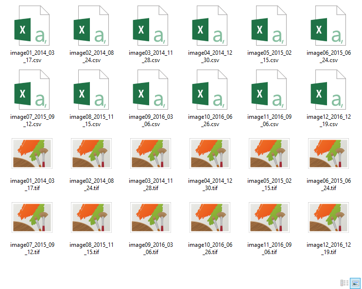
The whole dataset for MC3 contain 12 csv files and 12 tif files.
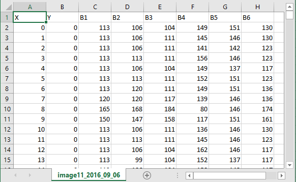
For csv file, each file contains coordinate information and band values for particular date, which is shown below:
This csv file contains all information on Sep "2016-09-06" and other 11 csv files are with the same format
Tools
R
Data Consolidation
First of all, we need to combine all 12 image data into one consolidated file, which is necessary for the following analysis.
The following R code shows the process of data consolidation including adding more columns for their "Date".
Adding Region Clustering
After using relevant measurement to define the property of certain regions on a particular date, we need to apply it for all dates.
We export the clustered Region data into csv file and use R to duplicate it for all dates.
JMP
Imagedata
After consolidating the data, there are more than 5 million records in the dataset, which is above the limit of Excel.
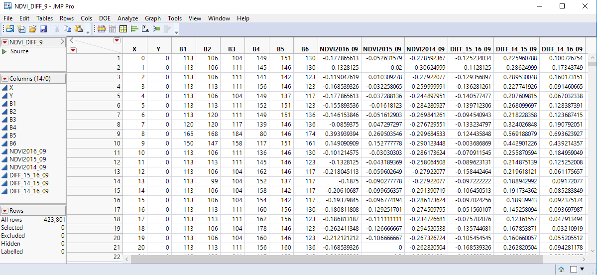
So we use JMP to view and modify the data. What shown below is the consolidated dataset.
NDVI difference
In order to see whether there is obvious change of Plant Health between 2016 and before, we calculate the difference of NDVI between (2016 and 2014) and (2016 and 2015).
We import data into JMP and use formula to calculate the difference between two particular dates.
Tableau
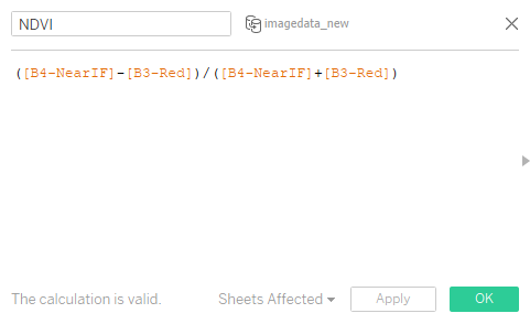
Calculated field
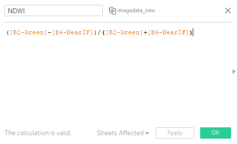
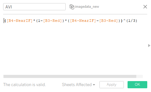
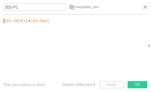
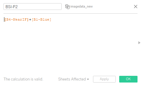
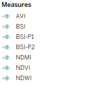
In order to discover the features and better evaluate particular performance, we need to use Calculated Field to create more measurements including NDVI, NDWI, NDMI, NDSI, AVI, BSI, etc.
Bin
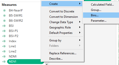
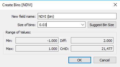
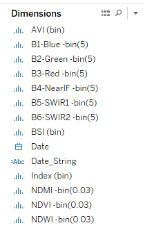
In order to see the distribution of each band and measurement from the histogram, we need create bin for them. Otherwise, they are continuous variable which can not reflect the accurate distribution.
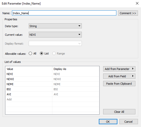
Parameter
In order to offer a better interaction to users, we need to create parameter for different measurements. This interaction allows users to choose different measurement and its related graphs in a single dashboard.

