ISSS608 2016-17 T3 Assign JOSEF CARLO CUEVAS EXCONDE FACTORY
ISSS608 Visual Analytics and Applications
|
|
|
|
|
WHERE DOES IT COME FROM?
The last question in the 2nd Mini Challenge for VAST 2017 focuses on among the 4 factories who uses the data, we can do this by interpolating the values from the sensors to our known coordinate of our factories and by comparing the interpolated values between the factories we can conclude that whoever has the highest reading would be the one responsible for the chemical.
Tableau Public Link : https://public.tableau.com/profile/josef.carlo.cuevas.exconde#!/vizhome/FactoryReadings/FactoryReadings
Data Preparation
For this part of the Mini Challenge, I opted to prepare the data in JMP Pro 13 by using the Sensor Reading Data and the Coordinate of both the factories and the sensors. From the given data we can refer to the following coordinates:
Factory Coordinates
- Roadrunner Fitness Electronics: 89,27
- Kasios Office Furniture: 90,21
- Radiance ColourTek: 109,26
- Indigo Sol Boards: 120,22
Sensor Coordinates
- Sensor 1: 62,21
- Sensor 2: 66,35
- Sensor 3: 76,41
- Sensor 4: 88,45
- Sensor 5: 103,43
- Sensor 6: 102,22
- Sensor 7: 89,3
- Sensor 8: 74,7
- Sensor 9: 119,42
A new 16 row table would then be prepared that would include the combination of the 4 factory names together with its X and Y Coordinates, the chemicals . Another action needed to be taken is splitting the Sensor Reading Data by setting Split By to Monitor and Split Column to Reading After that we can perform a Table Join by matching the Chemicals on the new table and the Sensor Reading table. On the new table we would need to compute for the distance between the sensor and the factory using the formula below.
After this we would have 9 new column(R1 - R9) with each showing the distance between the factory and the sensor. After that we can use the Inverse Distance Weighting formula to compute for the reading at a given factory.
Where:
Z = Factory Reading
S = Reading at the Sensor
Factory Reading
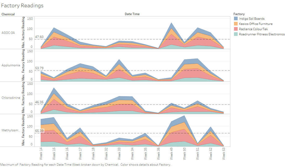
Finally we can transport the dataset from JMP to Tableau by saving it as an *.xlsx then reloading it to create a viz. To be able so satisfy the requirement of the mini challenge question 3 we would have to look at the data as a time series which would be showing its operation pattern for the 3 month worth of sample data. We could look at this data from 2 perspective, a continuous time series representation to see if there is any change in the reading per factory through time or compare each specific time period(i.e day of the week) per week to see if there are any patterns specific to each day through the observed time series.
First Graph
Column Shelf : Week(Day Time)
Row Shelf : Chemical @ Max(Factory Reading)
Mark Card
- Graph Type: Area
- Color : Factory
Second Graph
Column Shelf : Weekday(Day Time) & Week(Day Time)
Row Shelf : Chemical @ Max(Factory Reading)
Mark Card
- Graph Type: Area
- Color : Factory

