AY1516 T2 Group 18 Project Findings
Contents
Logistic Regression
In hopes of identifying the significant factors that affect consumers’ decision on buying Personal Care products, we employed the use of a logistic regression model. A logistic regression model was used due to the categorical dichotomous nature of the response variable. In addition, the relationship between the independent explanatory variables and the dependent response variable is also not linear, which violates the assumption of a linear regression model.
Dealing with Multicollinearity
Before performing logistic regression, we had to check for multicollinearity amongst all of the variables. This was important to administer because logistic regression is sensitive to extremely high correlation among independent variables, which would give rise to a large standard error for parameter estimates. This was done via a measure of association between all (categorical) variables. We looked at the Lambda and Uncertainty measures as indicated in Figure 14 to determine if the categorical variables are highly associated with each other. We dealt with variables with high correlation with each other by eliminating one or more redundant independent variables from the model. We made sure that the correlation among the explanatory variables do not exceed a maximum coefficient of correlation of 0.5 before proceeding with our logistic regression analysis.
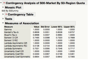
Figure 14: Measures of Association table for example variables Market and Region
Dealing with “Missing Values”
Some of the questions in the survey are asked or skipped based on a respondent’s answer for the previous question. For example, if the answer to the question “In regard to device and media usage, was yesterday a typical day for you?” is “yes”, then the next few questions in the survey would be asked. Otherwise, the questions would be skipped. Figure x is shown below for a clearer understanding of the scenario:
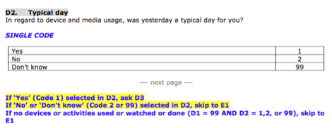
Figure 15: Example of a question showing routing rules
As a result of such questions, there were areas in the dataset indicated as missing values, simply because the questions were skipped for certain respondents. With the missing values in place, logistic regression will only evaluate the rows without any missing values. Hence, our results will suffer should there be a large number of missing values present. In order to deal with the missing values, we could either exclude the rows with missing values entirely, or do imputation. However, due to the large number of missing values (over 300 responses at an instance), we could potentially miss a lot of information from these respondents should we exclude it or replace it with another value. Hence, we replaced the missing values in two ways:
- For continuous variables, we converted the responses into categorical variables instead, with 4 measures - “not a typical day”, “did not use this service”, value less than median, and value more than median, where the median was determined after excluding the missing values
- For categorical variables, we replaced the missing values with “not a typical day”
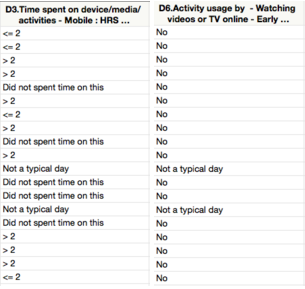
Figures 16 and 17: resulting categorical variables after dealing with missing values
Modelling Strategy
We employed the use of the Stepwise function in the Fit Model platform of SAS JMP Pro 12 to build the explanatory model for Personal Care consumers. Since we have a large number of variables at hand, we chose to use Stepwise since it is often used to reduce the number of variables. We changed the direction to “Mixed”, at the 0.05 level of entry and exit. The Mixed option combines the Forward and Backward direction option, so it tends to lessen the magnitude and likelihood of possible interpretation and prediction errors, since variables are evaluated twice in the process, where variables can be dropped after they have been added. An advantage of the Stepwise function is that it is an automated algorithm, hence, it is fast and easy for us to build the model.
However, a limitation of JMP prevented us to evaluate all possible explanatory variables at once. As a result, we needed to split the variables and run the Stepwise function separately based on their sections to drop initial variables that are insignificant. Finally, we combine all variables left in each section in our final model.
Evaluation of Logistic Regression Model
Performance of the Logistic Regression Model
We assess the overall performance of our logistic regression model using several different measures - the whole model test, misclassification rate, confusion matrix, and the Receiver Operating Characteristic (ROC) curve.
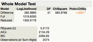
The hypothesis for the Whole Model Test is:
Since our results indicate that p-value < 0.0001 shown in Figure, there is sufficient statistical evidence to reject the null hypothesis. Therefore, we can conclude that the logistic model is useful to explain the odds of the Personal Care consumers. In other words, the overall model is significant at the 0.0001 level according to the Model Chi-Square statistic.
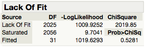
In addition, we use the Lack of Fit test (i.e. Goodness of Fit) to evaluate if our model is adequate to explain the odds of Personal Care consumers. We form the hypothesis as follows:
Since our results show that the p-value = 0.5281 ( >0.05 ), there is insufficient evidence to reject the null hypothesis at the 95% confidence level. Therefore, we can conclude that our logistic regression model is adequate and that there is little to be gained by introducing additional variables to the model.
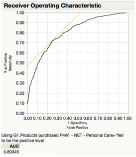
The ROC curve, which is a plot of sensitivity by (1-specificity) for each value of x, with a value of 0.80345, indicates that there is very good distinguishing ability in identifying Personal Care consumers from the model.
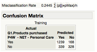
Lastly, the misclassification rate for our logistic regression model is 0.2445. This rate can also be derived from the confusion matrix table above, there are 339 false positives and 168 false negatives. Therefore, the overall misclassification rate works out to be 24.45% (i.e. (339+168)/2074). We can conclude that according to the misclassification rate measure, our model is able to predict 75.55% of the Personal Care consumers correctly.
Overall, based on the misclassification rate, confusion matrix, whole model test, lack of fit test, and ROC curve, we can draw the conclusion that the performance of our model is good for explaining the odds of Personal Care consumers.
Performance of the Individual Parameters
After we have established that our model is sufficient in explaining the odds of Personal Care consumers, we need to assess the individual parameters to sieve out significant explanatory variables that identify Personal Care consumers. We use the Likelihood-Ratio Tests (LRT) to help us with that. While the logistic regression output in SAS JMP Pro 12 provides the results from the Parameter Estimates based on Wald’s tests, we use the LRT instead because LRT tests are computed iteratively, and hence, would produce more reliable results.
The table below is a summarization of the results based on the different categories:
| Category | Explanatory Variable | Significance Level |
| Demographics | Gender | <0.0001 |
| Household Income | ||
| Employment Status | ||
| Section B: Device Ownership | Owns: Pay-TV subscription | <0.01 |
| Intends to buy: Nothing | ||
| Mobile brand | ||
| Mobile service provider | ||
| Section C: Digital Activities | Freq. of online activities: reading news, sport or weather | <0.01 |
| Freq. of online activities: mobile payment | ||
| Freq. of online activities: upload photos, videos, or music | <0.05 | |
| Section D: Daypart Usage | Online shopping | <0.01 |
| Read newspapers/magazines in the early evening | ||
| Don’t know which part of the day listen to the radio | ||
| Social networking during dinner | ||
| Don’t know which part of the day Shopping & Researching online | <0.05 | |
| Watch videos or TV online in early morning | ||
| Section E: Category Engagement | Engages online by - Reading emails from brands | <0.01 |
| Willing to engage with online - Government services | ||
| Willing to engage with online - Cosmetics or skincare | ||
| Prefer to use - YouTube to find out info about a brand | ||
| Engages online by - Comment or share brand posts on Facebook | <0.05 | |
| Prefer to use - WhatsApp to access entertainment content from or about a brand | ||
| Section F: Digital & Social Segmentation | Seek advice from social networks / official information | <0.05 |
Decision Tree
Another multivariate analysis that can help us to identify the significant factors that affect consumers’ decision on buying Personal Care products is using the decision tree method in recursive partitioning, a classification technique. Decision tree is a hierarchical model composed of decision rules that recursively splits independent variables into homogeneous zones (Lee and Park, 2013), where the most important factor will be located at the root of the tree.
The decision tree method is different from the logistic regression method in that the decision tree, being a nonparametric approach, does not require any statistical assumptions concerning the data. In addition, it can also handle incomplete and qualitative data. In terms of these two aspects, decision tree proves to be at a more advantageous position as compared to logistic regression because firstly, such assumptions are not always met in real world situations, and secondly, it is able to deal with the missing values identified in the previous section.
Modelling Strategy
Unlike logistic regression, we did an additional step to sieve out statistically significant variables at the 0.05 level through the Likelihood Ratio and Pearson’s chi-squared tests. After which, we ran our analysis by launching the Partition method in the Modelling platform. We set the method to Decision Tree and input our response variable and explanatory variables. We start to perform splits to the data by evaluating the Logworth of the explanatory variables, where the split will take place at the variable with the highest Logworth. We continue to split the data until we observe the following: the plot of the R-Square against the number of splits plateaus, because this indicates that additional splits will no longer provide any additional value to the model; the Logworth of each additional variable following each split is no longer increasing as much; and the misclassification rate is no longer improving as much with each additional split. To prevent the tree from growing too big, we will prune the tree as long as we felt that the additional splits are not adding as much value to the decision tree anymore.
Evaluation of the Decision Tree Model
Performance of the Decision Tree Model
We used three measures to evaluate the performance of our decision tree model - misclassification rate, confusion matrix, and the ROC curve.
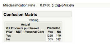
Figure 29: Confusion Matrix table for the decision tree model
The misclassification rate for the decision tree model is 0.2430. This rate can also be derived from the confusion matrix table above, where there are 355 false positives and 149 false negatives. Therefore, the overall misclassification rate works out to be 24.3% (i.e. (355+149)/2074). We can conclude that according to the misclassification rate measure, our model is able to predict 75.7% of the Personal Care consumers correctly.
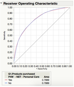
Figure 30: ROC curve for the decision tree model
The ROC curve for the decision tree model indicates a value of 0.7889. While this indicates that there is very good distinguishing ability in identifying Personal Care consumers from the model, the distinguishing power is lower than that of the logistic regression model.
Overall, based on the misclassification rate, confusion matrix, and ROC curve, we can draw the conclusion that the performance of our decision tree model is good for explaining the odds of Personal Care consumers.
Assessing Individual Parameters
| Category | Explanatory Variable |
| Demographics | Gender |
| Household Income | |
| Race | |
| Section B: Device Ownership | Mobile Service Provider NPS |
| Owns - Pay-TV subscription | |
| Owns - Smartwatch | |
| Owns - Tablet | |
| Section C: Digital Activities | Freq. of online activities - Reading news, sport or weather |
| Freq. of online activities - Listen to internet radio / music online | |
| Freq. of online activities - Visiting blogs or forums | |
| Freq. of online activities - Upload photos, videos or music | |
| Social / IM Usage - Facebook Messenger | |
| Section D: Daypart Usage | Online shopping |
| Watched TV | |
| Listened to radio | |
| Watched TV early morning | |
| Listened to radio in bed when woke up | |
| Section E: Category Engagement | Willing to engage with cosmetics / skincare online |
| Willing to engage with any brands online | |
| Willing to engage with mobile network operators | |
| Willing to engage with government services | |
| Prefer to use - access entertainment content from or about a brand Google+ |
Comparison of Logistic Regression and Decision Tree
Comparing confusion matrix:
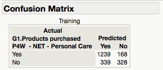
Figure 31 (left): Confusion Matrix for Logistic Regression model
File:Confusion matrix (desicion tree).jpg
Figure 32 (right): Confusion Matrix for Decision Tree model
.jpg)
Comparing misclassification rate - Logistic Regression: 0.2445, Decision Tree: 0.2430
Recommendations
Coming soon!
Limitations
Coming soon!
Conclusion
Coming soon!