ANLY482 AY2017-18 T1 Group2 Project EZLin Project Methodology
Current Approach
Currently J&J uses SAP software to manage its internal database. The data that they are able to provide for studying the supply chain includes the detailed cost components’ information for each product in each plant, plants’ description, raw materials’ information, the relationship of the shipments between different plant as well as the net trade sales data.
Before any further analysis on the data was able to be conducted, there were three main problems that we faced.
The first problem was that there was not a single excel file that contained all the necessary information, making it very difficult for us to initially use Tableau for our visualisation. For instance, the file containing material’s cost components are being separated into several excel files and in accordance to where they are manufactured or held in a distribution centre. In addition, to be able to trace the shipment flow with its respective information, the special procurement type excel file has to be referred to.
Secondly, due to JnJ’s internal data structure, the various cost components in the Bill of Materials (BOM) data are in hierarchical structure(Figure 1). If we use this hierarchical structure data to do the visualization directly, a lot of cost components will be double counted.
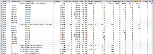
Figure 1 hierarchical structure data
Lastly, the table structure for storing the cost components is not very suitable in doing visualisation. This is because the origin structure has numerous rows of cost components and each rows contains all the cost components value for one material. This results in having numerous cells with 0 value as there is no cost under that particular cost component.
Given these, there was a need to process and transform the data in order to come up with some form of visualisation.
Data Transformation
Techniques we used for data transformation is python. Libraries we have used include pandas, numpy, itertools. Pandas contains a lot of functions which make data transformation easier. And itertools is for looping through the whole data set.
Firstly, we combined all excel files containing detailed cost component information(Figure 2,3). This included the Manufacturing BOM file, the Distribution Centre (DC) BOM file as well as the Subcontractor (Subcon) BOM file. Without combining all the excel file, it will be difficult to visualise all the information together.
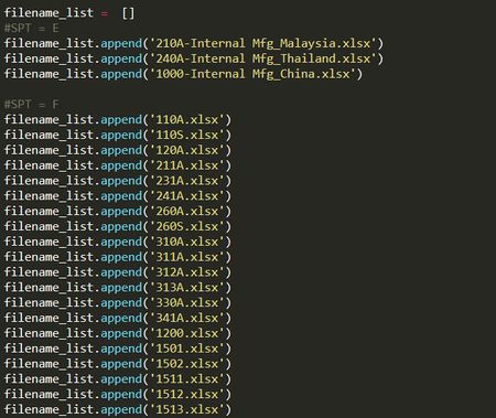
Figure 2 add all excel files into a list
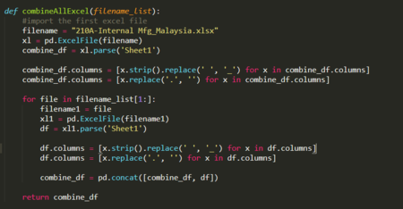
Figure 3 combine all excel files
Following the consolidation of the BOM files, in order to let each material maintain and keep track of its hierarchical relationship in one BOM, a SerialCode column and Bom_Id column was added(Figure 5,6). For example(Figure 4), if one Level 3 material’s material no is OHDIR and its parent material no is 8008608 for level 2, 28001426 for level 1, then the SerialCode for this specific material is 28001426/8008608/OHDIR. Its Bom_Id is 28001426, which is the Level 1 material’s material no of this bom.
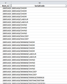
Figure 4 example of SerialCode and Bom_Id
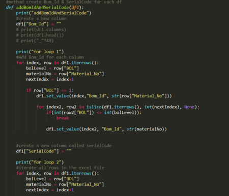
Figure 5 add Bom_Id and SerialCode
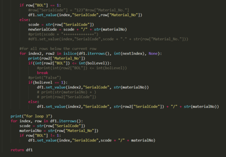
Figure 6 add Bom_Id and SerialCode
Once the BOM cost components has been properly structured, there was a need to map the shipment flow of the product by seeking the original plant for each material. To do so, we merged the combined excel file (containing all the cost components) with material master.xlsx file to get the Special Procurement Type (SPT) for each material(Figure 7). The SPT is a key denoted by alphabets and numeric value, each representing where was the product shipped from. With the SPT and plant of the material, we can join the table with Special procurement type description.xlsx to get the Long Text which contains the original plant no(Figure 7). Then, using some python string methods, we get the exact plant code from Long Text(Figure 8). (eg. Stock from(210A) -> 210A).
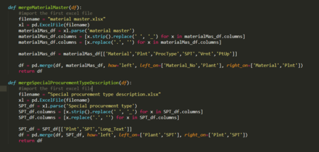
Figure 7 merge the combined excel file with material master.xlsx to get the SPT & get the long Text from Special procurement type description.xlsx

Figure 8 get the origin plant no from Long_Text
Given the variety in volume and types of product available, each material’s Putup (product volume) information and Variant (product type) information were also important for the comparison of the cost and components. As such, the consolidated table based on the above mentioned consolidation was also joined with the putup.xlsx and variant.xlsx(Figure 9).
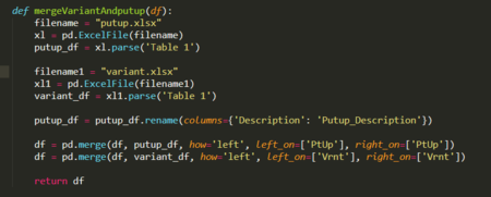
Figure 9 join the combined excel with putup.xlsx and variant.xlsx
Based on the requirements of JnJ, it was essential that there was uniformity in the comparison which meant that the products had to be compared using the same unit. From the original BOM files, the raw data’s cost values were all in different currencies and in different product volume due to the large variety of products. The sponsor thought that it would be preferable to compare all the materials in either 1 Litre (L) or 1 Kilogram (KG) so that the comparison would be meaningful. Therefore, we transformed all the cost values to USD(Figure 10) and the volume into 1L / KG(Figure 11).

Figure 10 transform all cost values to USD unit
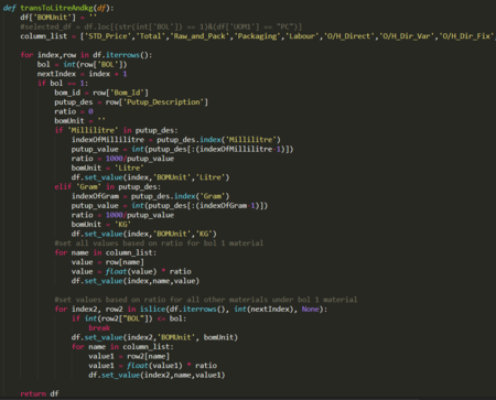
Figure 11 transform all cost values to Litre(or KG)
For the transposition of data, we needed to make all the materials that are in the same bom to have the same original plant, variant description and putup description(Figure 12).
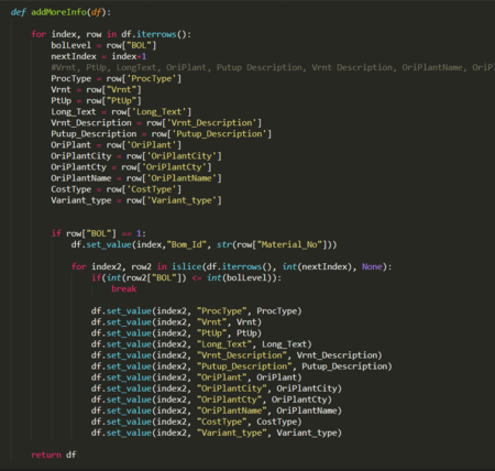
Figure 12 add the same information for each material in one BOM
Following that all BOM materials to have the information, to avoid double counting materials, the rows that were not at the bottom level of the BOM had to be deleted(Figure 13). Only with this was it possible to transpose the data(Figure 14,15), which is to create rows reflecting the different cost components for one material.
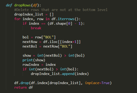
Figure 13 drop rows that are not at the bottom level of the BOM
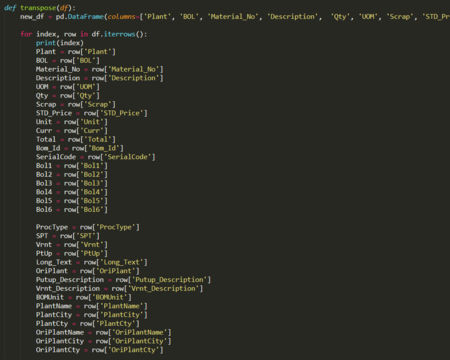
Figure 14 transpose for each material in the BOM

Figure 15 transpose for each material in the BOM
Lastly, to incorporate more information and to derive more insights about the packaging cost as well as the raw materials’ cost, the consolidated table above was merged with the Packaging Data.xlsx and ChemicalWithPlantCode.xlsx(Figure 16).
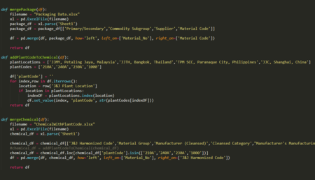
Figure 16 merge the combined file with packaging file and chemical file
Visualization and Report Generation
We visualised the information using tableau with various functions in the software, and presented the data through charts, dashboards and story format.
To visualise the data, we imported the consolidated table with all the information we needed into Tableau. In order to clearly see the difference in cost between different countries, plants and types of product, a calculated field known as “Average Cost Amount” was created using edited field in Tableau. This is because the consolidated data table included only the lower level products. By summing up all the BOLCost value and dividing by the number of unique Bom Id and number of unique Plant number, it will give us the average unit cost. (Figure 17)

Figure 17 Average Cost Amount (USD/Liter) formula
1.1 Manufacturing Cost
To compare the difference between manufacturing cost in different countries, we placed Average Cost Amount under Columns and Variant type, Putup Description and Plant Cty under Rows (Figure 18). By filtering the Procurement Type to “E” only, which stand for internal manufacturing cost, only the manufacturing cost was being reflected. Based on this, we can compare the difference in manufacturing cost for the same product of the same volume, produced in different countries. For example, in Figure 19, we can conclude that the manufacturing cost of Body Lotion in China is relatively higher than the cost in Thailand. To view the details of the manufacturing cost, we used colours to differentiate the proportion of BOL cost (Figure 20). We can also filter and analyse the cost difference of different components in different countries such as labour cost, raw material cost and duty cost (Figure 21).
![]()
Figure 18 Manufacturing Cost Columns and Rows

Figure 19 Body Lotion manufacturing cost of various volumes and manufacturing countries

Figure 20 Lotion manufacturing cost component
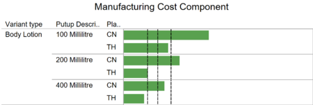
Figure 21 Labour cost in Lotion manufacturing cost
1.2 Distribution Cost
To compare the difference between distribution cost, one additional column Ori Plant Cty is placed in front of Plant Cty (Figure 22). By filtering the Procurement Type to “F” only, which stand for distribution cost, only the distribution cost would be reflected. For example, in Figure 23, we can compare the difference in distribution cost for Body Wash 750 millilitre that was being shipped from different origins to different distribution centers. The distribution cost differs when the same unit from Malaysia or Thailand is shipped to different distribution center. For instance, when shipping from Thailand to Singapore, the cost is higher than when the product is shipped from Thailand to Vietnam. And when the same product is shipped to Vietnam, the cost is higher when the origin is Thailand instead of Malaysia. Charts similar to Figure 4 and 5 is also created for distribution cost.
![]()
Figure 22 Distribution Cost Columns and Rows
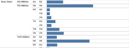
Figure 23 Body wash distribution cost of various volumes and manufacturing countries
1.3 Subcontracting Cost
The Subcontracting cost is relatively similar to the distribution cost. The only difference between this two is the filtering of the Procurement Type to “X” instead of “F” and filtering the Type of cost to “Subcon” cost. The reason for this is so that only the subcontracting cost are included and any duplicate records from either the manufacturing cost or distribution cost are completely removed (Figure 24).
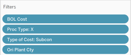
Figure 24 Filters of subcontracting cost chart
1.4 Dashboard
Following the creation of the different worksheets, we combined the overall manufacturing cost and manufacturing cost component into a single dashboard, the overall distribution cost and distribution cost component in another dashboard and the overall subcontracting cost and subcontracting cost component into a third dashboard (Figure 25). The reason for having three different dashboards is for easier visualisation for each type of cost and to allow for comparison between the overall cost with the different cost components. All three dashboards are then added into one storyboard using different tabs for easier visualization and storytelling. (Figure 26)
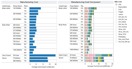
Figure 25 Manufacturing cost dashboard
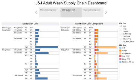
Figure 26 Distribution cost in Supply Chain storyboard
1.5 Chemical data
To view the cost of chemical used in various product, we used a storyboard similar to the supply chain storyboard (Figure 27), to connect dashboards which represent the chemical data cost comparisons (Figure 28).
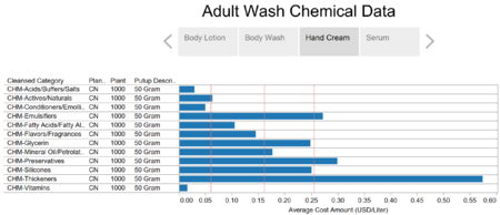
Figure 27 Hand Cream chemical cost in Chemical Data storyboard
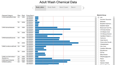
Figure 28 Chemical data storyboard
To compare the difference between chemical cost of the same product in different countries, we put Average Cost Amount in columns and Cleansed Category, Plant Cty, Plant and Putup Description in rows (Figure 29). The Material Group was used as a filter to look at the cost difference of that particular material group. For example, in Figure 30, we can conclude that the cost of chemical Ascobric Glucoside which belongs to Category CHM-Vitamins is relatively higher in Thailand than in China regardless of volumes of the product.
![]()
Figure 29 Chemical data Columns and Rows

Figure 30 Chemical cost of Ascobric Glucoside in CHM-Vitamins comparison
1.6 Packaging Data
We also used an individual dashboard to show the comparison of packing cost between different countries, through putting Average Cost Amount in columns and Primary/Secondary, Putup Description, Plant Cty, and Plant in rows. (Figure 31) And we colour the charts by verifying the Commodity Subgroup we see the comparison between packing cost of different component of finishing products. For example, in Figure 32, we can conclude that the cost spent to produce Caps/Closures/Lids is higher in China than in Thailand.
![]()
Figure 31 Packing data Columns and Rows

Figure 32 Packing Cost component
2.1 Supply Chain Cost
In general, the overall manufacturing cost in China is higher than the cost in Thailand and Malaysia based on the chart.(Figure 33) And in terms of volume, majority of the products have the same regularity which is the larger the volume is, the lower a unit of the product costs. The company could consider manufacturing more products in Thailand and Malaysia instead of China and produce larger volume of product instead of smaller volumes if possible.
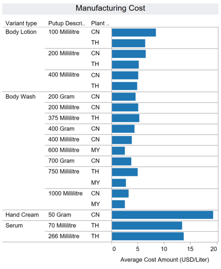
Figure 33 Overall Manufacturing Cost
The manufacturing cost in China is higher because its labour cost is around twice the labour cost in Malaysia and Thailand on average. (Figure 34) Although Thailand and Malaysia were called Tiger Cub Economies back in 2009, which implies that they are the few Asian countries that start their industrialization earlier than the rest. But it is obvious that their economic development is slowing down and they are exceeded by China therefore the labour cost in China is even much higher.
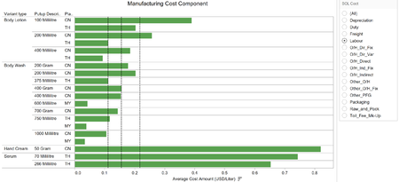
Figure 34 Manufacturing labour cost
But at the same time, we can analyse from the data that duty and freight cost of manufacturing in China is clearly lower in China compare to the other two countries. (Figure 35) For duty cost, an inference is that for domestic wise, the movement within China itself incurs less duty cost. This is because for duty wise, China has preferential duty reduction for five special economic zones (Shantou, Shenzhen, Zhuhai, Xiamen, Hainan), open cities and foreign trade zone (Guangdong, Fujian, Tianjin). While Thailand has generally higher duty due to their high tariffs in many sectors due to ad valorem, which is duty paid in proportion to the estimated value of the good or services.
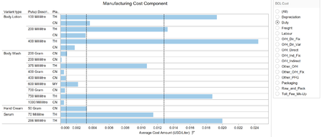
Figure 35 Manufacturing duty cost
The company could also look through their Distribution Cost due to inconsistency in some of the costs. For example in terms of freight cost, for Body Lotion 200ml, it can be seen that the trip from Thailand to Malaysia is more expensive than Thailand to Japan or Taiwan. This is even though geographically, Thailand is closer to Malaysia than Thailand is to Taiwan. Similarly, for Body Wash 750ml and 1000ml, the freight cost from MY to HK falls into the lower quartile and it’s almost on par with MY to SG, which is geographically nearer (Figure 36).
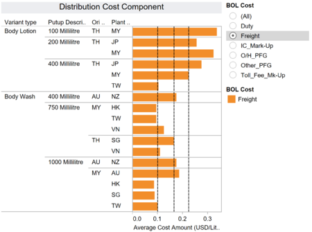
Figure 36 Distribution freight cost
2.2 Chemical Data
Generally there is no clear trend as to which country is more expensive in terms of chemical cost. For example, under Body Lotion, for chemical Chamomilla Recutita and Chlorphenesin, the cost in China is about twice the price of Thailand. (Figure 37) On the contrary, for chemical Citric Acid, the cost in Thailand is about twice the price of China. (Figure 38) As such, there is no clear indication in terms of trend for the chemical data.

Figure 37 Body Lotion chemical Chamomilla Recutita cost

Figure 38 Body Lotion chemical Citric Acid cost
The regularity of volume is that the larger the volume of product the cheaper the chemical is. But there are contrarian cases as well. For example, for the chemical Butylated Hydroxytoleune in Body Wash, the larger the volume the more expensive the chemical is (Figure 39).

Figure 39 Body Lotion chemical Butylated Hydroxytoleune cost
2.3 Packing Data
For Body Lotion primary packing data, the cost variation around different countries are generally the same. For some, it is more expensive in China while for others, it is more expensive in Thailand. In terms of types of packaging, it is generally cheaper to produce the primary packaging, which includes the main bottle, but more expensive to produce the caps or the lids in China. For Thailand, it is more expensive than China to procure/produce for the Secondary packaging. So it’s more expensive to produce in Thailand.
In terms of the Subgroup for the packaging, Thailand has an additional “Other Packaging” that is not available in China, which makes the packaging more expensive with the additional cost (Figure 40). And this applies to the other types of products as well.

Figure 40 Body Lotion Packing data
Limitation
Over the course of this practicum, the team faced many limitations and challenges in trying to derive insights from the dataset.
One of the main limitation faced in deriving our insights was the constant change in the raw data set. Due to the insufficient understanding and knowledge of the data by JnJ, our team was either presented with new dataset or new way of interpreting the data every meeting. This resulted in much confusion and us needing to retransform our data for our visualisation. Given the short span of the project, this constant re-iteration greatly reduces the time we were able to spend deriving insights and mapping the end-to-end flow.
Another limitation faced by the team was the insufficient experience and knowledge with regards to Analytics. Even though we did take some course (e.g. Data Mining, Visual Analytics etc.), we are not fully equipped with the required knowledge and expertise in the transformation as well as the visualisation of the data. This often cause us to spend much time in structuring the data and in visualising the data to reflect meaningful insights for JnJ.
A third limitation faced by the team was the incomplete data provided by the company. Some of the raw data files provided by the company was insufficient and did not provide a true representation of the supply chain network. For example, the packaging and chemical data provided by the company was not comprehensive and contained insufficient information. This undermined the visualisations and insights derived as the data itself did not accurately reflect the actual information.
All in all, more could have been done to derive not only the insights but also map the end-to-end supply chain flow as required by the business unit. However, given the limitation in the project timeline and the inadequate knowledge in Analytics as well as the related software, the visualisations and the insights were our main deliverables for the client.
Conclusion
In conclusion, we tried to derive insights based on the understanding of the data. However, much transformation and processing of the raw data was needed before any visualisation could be done or insights to be derived. From the data transformation and Tableau visualisation, we were able to conclude that the data had numerous quality issues which made the analysis inconsistent. Furthermore, the incomplete and static dataset compromise the actual reliability of the insights. Despite this, it was definitely beneficial for the sponsor to truly understand and have a clear picture of how such quality issues truly affects the data reliability.
Even though Python was the primary language used for the project, we acknowledge that R may have been better in the consolidation and statistical analysis of the data. However, due to the limitation in time and the familiarity with Python, it became the primary choice for this project.
Although many of the initial requirements of this project was not fully met, nonetheless to be able to automate the data cleaning process through the code and highlight the data quality issues is a step forward for JnJ in its push towards leveraging on analytics.