Automotive Angels - Analysis
Contents
- 1 Analysis
- 1.1 Exploratory Data Analysis
- 1.1.1 Relationship between Current Selling Price and Current Suggested Retail Price
- 1.1.2 Relationship between Current Selling Price and other variables
- 1.1.3 Number of listings by dealer
- 1.1.4 Relationship between Current Selling Price and Corrected Vehicle Models
- 1.1.5 Vehicle Models by Frequency and Current Selling Price
- 1.2 Application of Methodology
- 1.3 Results
- 1.1 Exploratory Data Analysis
- 2 Discussion
Analysis
Exploratory Data Analysis
For data exploration, we will be conducting exploratory data analysis. Exploratory data analysis includes the following steps:
- Analyzing the distribution of variables
- Treating outliers that were identified
- Compare models’ “Current Selling Price”
- Examine relationships between variables
- Develop hypotheses based on literature and hypothesis testing
Relationship between Current Selling Price and Current Suggested Retail Price
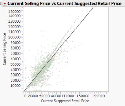
Before plotting a scatterplot, we removed the extreme outliers from “Suggested Retail Price” to get more detailed scatterplot. Extreme outliers are more than 3 times of the interquartile range past the tail quantile and 1- tail quantile where the tail quantile is defined as 0.1. From the Figures below, “Current Selling Price” is strongly correlated to “Current Suggested Retail Price” with a R2 of 0.888 (Figure 9) for BMW. This shows that “Current Suggested Retail Price” is a good predictor of “Current Selling Price” of Used Cars.
Figure 9: Scatterplot of Current Selling Price and Current Suggested Retail Price for BMW
Relationship between Current Selling Price and other variables
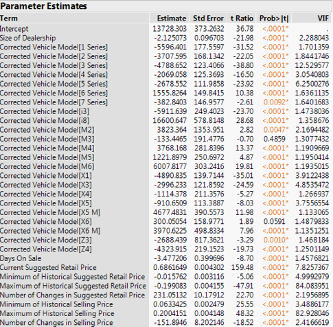
Figure 10: Parameter estimates based on fit of least squares for BMW
From the results of the fit of least squares in Figure 10, we know that the “Maximum Historical Suggested Retail Price” have a high VIF value of close to 84 and “Maximum of Historical Selling Price” have a high VIF value of 82. As such, there is multicollinearity and we will take it out to reduce noise and redundant predictor variables.
Number of listings by dealer
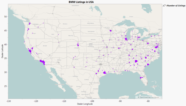
We can see that most of the used cars listed from BMW (Figure 11) listings are mostly from the East of North America other than some areas of concentration in cities in the East. One reason might be that more data is collected from dealers situated in the East of North America.
Figure 11: Map of BMW Dealers’ locations by Number of Listings for BMW
Relationship between Current Selling Price and Corrected Vehicle Models
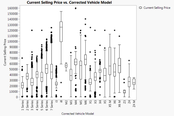
Figure 12: Box Plot of Current Selling Price by Corrected Vehicle Model for BMW
From Figure 12, we observed that there are models which have high median price as compared to other models such as i3 and i8. Also, we observed that models such as X5 and X5 M have significantly different prices as well and hence although both models are similar, it should not be merged as the same model.
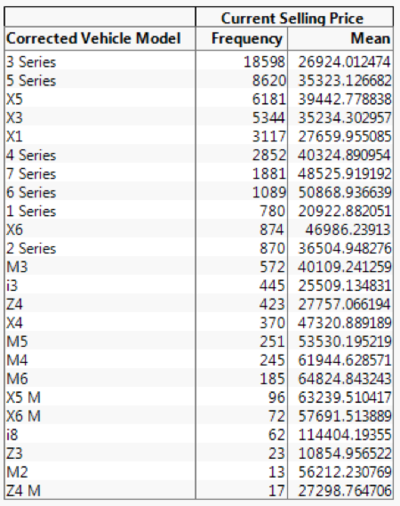
Vehicle Models by Frequency and Current Selling Price
Figure 13: Table of Corrected Vehicle Models by Number of Rows and Mean of Current Selling Price for BMW
We decided to choose the top 4 models to focus on in terms of frequency. They are: 3 Series, 5 Series, X3 and X5. From Figure 11, these 3 car models have similar price range of between 26000-36000USD.
Application of Methodology
According to Figure 3: Process Flow Overview, below the detailed steps taken at each stage.
- Filter out “Car Make” = BMW from the full dataset.
- Filter out “Used Status” = 0 from the remaining dataset since we are only predicting at used cars.
- Filter out “Vehicle Category” = ‘Not Car’ from the remaining dataset since we are only predicting cars.
- Filter out extreme outliers (Interquartile Range Multiplier = 3, Tail Quantile = 0.1) for “Current Selling Price” and “Vehicle Mileage”.
- Filter out 99995 < “Current Selling Price” < 99999 since those are likely to be wrongly recorded, as seen in the exploratory data analysis.
After the data is prepared, we can pass it through the above process flow shown in Figure 49 in the appendix:
- Data Import – we imported the prepared data into the process flow.
- Data Partition – we would be partitioning it randomly at 60% training data and 40% testing data to help prevent overfitting compared to 70% training data and 30% testing data, as said previously.
- Filter out each “Vehicle Model” – We will be creating a regression equation customized to each vehicle model.
- Filter out extreme outliers of below the 10th percentile and above the 90th percentiles. This also filters out “Current Selling Price” that are close to 0 which is unlikely because used cars would not be listed for no value.
- Linear regressions using 3 methods – Stepwise, Backward and Forward. We also include an option to minimize the difference in errors between the prediction result from train and prediction result validation using cross validation.
- Model selection helps us to choose the best model for linear regression based on the least mean squared errors.
Results
Using the same methodology, we redid the same steps for other vehicle makes, Ford and Chevrolet, and the results are as follows.
Results Summary
| Vehicle Model | Median | Min | Max | RMSE Train | RMSE Test | Adjusted R2 | Chosen Regression Model |
|---|---|---|---|---|---|---|---|
| Ford Focus | 11625 | 6600 | 17999 | 1248.25 | 1672.34 | 0.7824 | Forward |
| Ford Explorer | 25971 | 7995 | 35000 | 2179.76 | 3070.73 | 0.9431 | Forward |
| Ford Fusion | 14871 | 8750 | 20437 | 1204.1 | 1594.91 | 0.8595 | Stepwise |
| Ford Edge | 20996 | 11200 | 32880 | 2108.81 | 2500.24 | 0.8987 | Stepwise |
| Chevrolet Equinox | 16998 | 10996 | 23898 | 1199 | 2647.01 | 0.8335 | Stepwise |
| Chevrolet Malibu | 13998 | 8000 | 18878 | 892.84 | 1942.97 | 0.8771 | Forward |
| Chevrolet Cruze | 12599 | 9000 | 15998 | 844 | 2362.063 | 0.7876 | Forward |
| BMW 3 Series | 25993 | 18888 | 36840 | 2859.33 | 3292.121 | 0.8608 | Forward |
| BMW 5 Series | 34994 | 23981 | 47600 | 2941.032 | 3352.48 | 0.8733 | Stepwise |
| BMW X3 | 35811 | 25982 | 45645 | 2612.88 | 2874.16 | 0.8856 | Backward |
| BMW X5 | 42991 | 23995 | 55981 | 2108.81 | 2500.24 | 0.8556 | Stepwise |
Figure 14: Table of Summary of Results from Regressions
| Vehicle Model | Effects of Chosen Regression Model |
|---|---|
| Ford Focus | Intercept, Current_Suggested_Retail_Price, Vehicle_Model_Age |
| Ford Explorer | Intercept, Current_Suggested_Retail_Price, Number_of_Changes_in_Selling_Price, Number_of_Changes_in_Suggested_Retail_Price, Vehicle_Model_Age |
| Ford Fusion | Intercept, Current_Suggested_Retail_Price |
| Ford Edge | Intercept, Current_Suggested_Retail_Price, Dealer_State, Vehicle_Model_Age |
| Chevrolet Equinox | Intercept, Current_Suggested_Retail_Price, Vehicle_Mileage, Vehicle_Model_Age |
| Chevrolet Malibu | Intercept, Current_Suggested_Retail_Price, Number_of_Changes_in_Selling_Price, Number_of_Changes_in_Suggested_Retail_Price, Vehicle_Mileage, Vehicle_Model_Age |
| Chevrolet Cruze | Intercept, Current_Suggested_Retail_Price, Vehicle_Model_Age |
| BMW 3 Series | Intercept, Current_Suggested_Retail_Price, Vehicle_Mileage |
| BMW 5 Series | Intercept, Current_Suggested_Retail_Price, Days_On_Sale, Dealer_City, Vehicle_Model_Age |
| BMW X3 | Intercept, Current_Suggested_Retail_Price, Days_On_Sale, Dealer_City, Number_of_Changes_in_Selling_Price, Number_of_dealers_in_50_miles, Number_of_similar_cars_in_50_miles, Size_of_Dealership, Vehicle_Mileage, Vehicle_Model_Age |
| BMW X5 | Intercept, Current_Suggested_Retail_Price, Dealer_City Dealer_State, Number_of_Changes_in_Selling_Price, Number_of_Changes_in_Suggested_Retail_Price, Vehicle_Model_Age |
Figure 15: Table of Summary of Effects from Regressions
From our results, we observed the best performing model to be Ford Fusion with a RMSE of 1248 for Train and 1672 for Test. The difference of approximately 400 between train and test set shows good predictability of the model. The results also show that for some models, there are signs of overfitting, such as Ford Explorer and BMW X3 where we observe high adjusted R2 of 0.88 and above. Also, the variable selection for various models vary individually which suggested that a generalized model with common pool of predictors was not suitable. The results also show that the Current Suggested Retail price offers a good base for price prediction, and common predictors are Days on Sale, Vehicle Model Age and Vehicle Mileage. Effects of depreciation are observed where models incorporated Vehicle Model Age and Vehicle Mileage as predictors. Further explorations can be done on Days on Sale with Current Selling Price. Specifically, for BMW, we observe that the created variables such as Number of dealers in 50 miles and Number of Similar Cars in 50 miles are selected as predictors in BMW X3, which propose that effects of competition and geographical location affects pricing in certain models.
Discussion
Technical Discussion Analysis
In general, we found that creating a generalized model for all makes or models does not serve as a good predictive model due to the large RMSE. Hence, modelling should be done on a specific vehicle model. Also, within each model there may be iterations such as X5 and X5M which have significant differences and hence should not be rolled up to be the same model. This poses a difficulty as it will be costly to model different car makes as there are many and increasing number of car models released each year.
Ford
From the above results, it seems that we have a workable model. Our errors are relatively low at about R2 of 0.85-0.9 and RMSE of between 2000-3000. Our residual plots also show a good spread around 0. However, there is room for improvement for Ford Edge and Ford Explorer as there are some extreme outliers. There is also a slight heteroscedasticity which is more obvious in Ford Focus. Most of the residue also seems to be negative which means that the predicted value is more often higher than lower compared to the actual value.
Chevrolet
From the above results, the model shows an adjusted R2 ranging from 0.79 to 0.88. The model seems to be a good fit for each specific model. Also, the RMSE shows that error ranges from 2000 to 3000, and given the median price is within the band of 12000-16000USD, such variance is considered acceptable.
BMW
For BMW, we see an RMSE ranging from 2000-3000. Considering that the prices are ranged from 25000-43000USD, such price margin for a predictive model is small. In addition, the adjusted R2 ranges from 0.85-0.89 where it shows goodness of fit. However, looking at the residual plots, it seems to indicate patterns that show biased results, especially for BMW X3 as shown in Figure 55. A very clear horizontal line maybe since the current selling price crawled from the websites could be a specific selling price approximation by dealers.
Managerial communication on Analysis
The comments given by Steve Greenfield, CEO of Automotive Ventures, was that “This looks very impressive! Nice work, team!” In communicating with David Chisnell, the resident Data Scientist for Automotive Ventures, he mentioned that “On nearby and far dealers, especially the dealers beyond 50 miles and less than 100 miles, we had been assuming they were too far away to matter but may revise that based on your work and change the production algorithm that handles all makes and models. It's one of the things I’d like to hear more about from the team. You've also started a conversation the business implications of using days to sell (meaning prices decline over time), and using number of price changes, (we read that as a suggestion they over-corrected, although it's also possible it's acting as a proxy for hidden information like cars with a bad car-fax or that smell like smoke take longer to sell and are more likely to be dropped in price). On Friday, I'd be interested if your team has thoughts on which factors are direct and which might be acting as a proxy. I also noticed there was a negative impact attached to historical suggested retail price and wanted to discuss how that was calculated. It's good work and helps make our business smarter!” Specific comments on analysis are not included in this paper due to time conflicts and organization changes in the company.
Recommendations for client
We recommend further exploration and validation before implementing the current workflow process in Automotive Venture’s business model. With the current work, the process steps and regression calculations will be exported out of SAS Enterprise Miner into a format where the programmers can implement in Python or Ruby. Existing data filters will reduce the computational power required to compute the optimal regression model for each vehicle model and predict a price range. However extensive data cleaning is required for other vehicle makes and pose an issue as data crawled daily may not be effectively clean and usable for analysis immediately. This will affect the selling proposition of the company whereby data used is not real time and requires going through time for processing.
