AY1617 T5 Team AP Methodology Finals

DATA COLLECTION

Our team made a trip to SGAG’s office to extract the video data from SGAG’s Facebook page (5 sets of data). The total number of video data point extracted was 299 for the year of 2016. However, after looking through the data set, we had come to realise that some data that are important for our analysis to meet the set objectives were missing. Therefore, we decided to manually log down the data ourselves by watching one year’s worth of data. Therefore, at the end of the day, we have 7 sets of data.

DATA INTEGRATION

The integration of 5 data sources is done to form up 30 over data columns for the main analysis.Our team used JMP Pro for our data integration process. Data were matched using Post ID. Post ID is a identifier dedicated to each post in Facebook. As all the data sets are from Facebook, the data can be joined together using the Post ID. As some of the data downloaded contain repeated columns like Permalink (Permanent Uniform Resource Locator), we selected the columns from the tables during the join process.

DATA CLEANING

OUTLIER
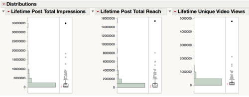
To clean the data, our group ran a distribution analysis on all the 299 data points to check for any missing or abnormal data. Upon doing so, we observed that there was a particularly high data point which could affect the data as seen in the figure below. After checking the data point, we then proceed to exclude it from our analysis.

Missing Data
Another observation was of instances of missing data where videos which were shared to SGAG’s Facebook page. As those posts were shared onto SGAG's Facebook Page, information such as the number of comments, likes and shares are not logging in SGAG's data set. Therefore, we proceed to exclude them as well.

Duplicated Data
Our team also checked the data for duplicate values and realised that there were actually two post which were duplicate. This have also been excluded from the data set.

Data Binning
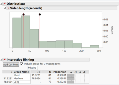
As the use of latent class analysis in SAS JMP Pro requires categorical variables for analysis, we had to bin one of ordinal our target variables (Video length). Our team made use of an add-in function called Interactive Binning, which allowed us to manually select cut-off points for the various bins. The video lengths distribution is then equally divided into 3 separate bins - Short, Medium and Long.

DATA PREPARATION

Month Column
To facilitate ease of analysis by year then by quarter, we added a month column, to allow us to easily filter out the months of the year to form the 4 quarters.

Johnson Transformation
In addition, our client has identified 4 key performance indicators (KPI) for the videos - the number of unique views, number of likes, number of shares and number of comments. As the ANOVA and Tukey-Kramer comparison test assumes a normal distribution, we were required to transform our key performance indicators so that they all follow a normal distribution. Our team has chosen to go with the Johnson family of transformation as it gives us much more flexibility, which in turn allows the data to be better fitted. The Johnson system allows a close approximation of a standard continuous distribution through one of its 3 functional forms SB,SU and SL.

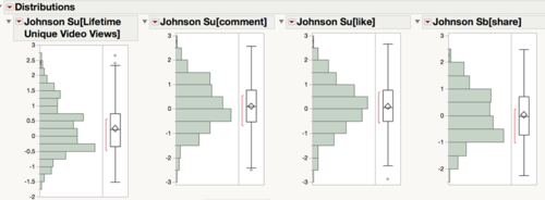
After performing the Johnson transformation, we then carried out a distribution analysis to check if the 4 transformed variables follow a normal distribution before we used them for further analysis, as seen from the figure below.

Principal Component Analysis
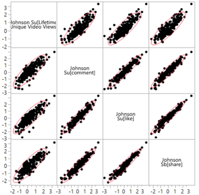
Since all 4 of our KPIs are highly correlated, there was a need for assigning an optimal weightage for each performance metric to derive a single differentiating metric for comparison.

Additionally, the 4 separate dimensions for video performance makes it difficult to compare across the videos, thus this further reinforce the need to reduce these dimensions into a single metric for comparability.

Our team utilised JMP Pro’s Principal Component Analysis (PCA), a dimension-reduction technique, to summarise the 4 video performance metrics into a single principal component. It works by constructing a new component based on the 4 video performance metrics using linear combinations to capture as much of the variability in the 4 video performance measures.

After performing the PCA, we generate the eigenvalues for our principal components which indicates the percentage of aggregate performance variation each principal component accounts for. We found that principal component 1 is able to account for close to 93% of the total variation in video performance, subsequently enabling us to utilise it for our ANOVA and Tukey-Kramer analysis.

Currently, we have the PCA done on the full year of data and by quarters to compare videos that were posted during the same time period. Additionally, PCA is also done on self-produced videos and videos starring the 4 main characters. Pairing PCA and Tukey HSD function, we were able to see which variables were doing better or worse than the others with 95% confidence and which variables does not seem to contribute to the videos’ performance (absence of P-value less than 0.05).

MODELS

ANOVA & TUKEY-KRAMER
The ANOVA model is used to conduct single factor studies on each video characteristics (e.g Tiers, genre, quality), corresponding to each factor level are the probability distribution of the video performance. For example, the effect of the videos being in different genre, how would it affect the final video performance metric as summarised previously by the principal component 1.

It is important to note the underlying assumptions when utilising the ANOVA model:

1. Assumes normal distribution in the data.

2. Each probability distribution has equal variance.

3. The responses for each factor level are random selections from the corresponding probability distribution and are independent of the responses for any other factor level.

LATENT CLASS ANALYSIS
Our group adopted the Latent Class Analysis to identify underlying unobservable subgroups. Latent class analysis is not only able to deal with different levels of clustering case variables and allowing us to handle missing data in almost trivial ways, it also is able to handle covariates and detects a non-cluster structure when it actually exists. The main reason why our team opted for latent class analysis over the conventional clustering methods is that it is a finite mixture model. It is able to derive clusters using a probabilistic model which describes the distribution of the data by making use of the conditional probability of our target variables’ response being observed in the cluster, as seen in Figure 17.

Our team first generated 3-5 clusters to determine the most optimal cluster number. When deciding on the cluster number, we observe the Bayesian information criterion (BIC) of the various models with different number of clusters formed. BIC is an estimated of a posterior probability that a model is true. The lower the BIC, the higher the probability that the model is considered a true model. Referring to the diagrams below, we can see that the Latent Class model producing 3 clusters has the smallest BIC value out of the 3 models. Therefore, our team has decided to analysis the data using a 3-cluster Latent Class model.