ANLY482 AY2016-17 T2 Group20 Findings
Data Exploration and Cleaning
Issues
Too large dataset
Due to the large dataset, it took too long to run the nodes in SAS Enterprise Miner which resulted in the inefficiency. It took approximately 6 hours to run a single node.
We reduced the dataset to BMW cars by filtering the dataset “makeName = BMW” and “used=1,2” to retrieve a dataset result of used BMW cars. We categorized the BMW cars based on the ‘modelName’, where the cleaning and categorization of ‘modelName’ will be explained below. Throughout the project, we will be using BMW cars as a model while keeping it generalised. Thereafter, we will be using the same model as a template for other car brands. This can be done by filtering the ‘makeName’ column which uses brand as the main filter.
This reduces the load on the system as we will only be using BMW cars for analysis.
Customers would already have a preferred car brand based on their buying capacity and personal preference for cars. From the general model, dealers will be able to select the car brands (“makeName”) of the customers’ preference, which will lead them to the specifications (“modelName”) of the car.
Unclean variable – modelName
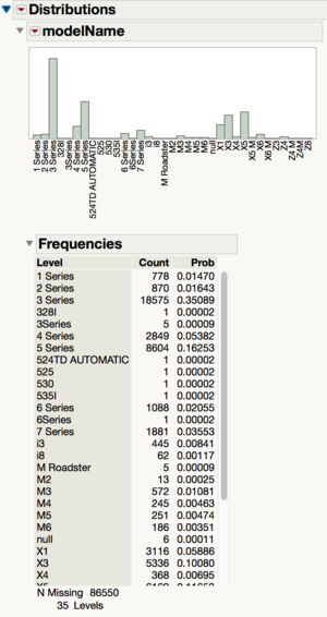
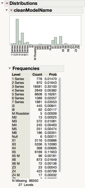
When we looked at the summary statistics of modelName, we can see that there are a few categories which should belong in another. For example, in the screenshot above, you can see that there are many 3 Series trims such as ‘318’, ‘323’, ‘325i’ which should belong in the ‘3 Series’ category so should be relabeled to ‘3 Series’.
Missing Values
| Column | Number Missing (before) | Percentage Missing (before) | Number Missing (after) | Percentage Missing (after) |
|---|---|---|---|---|
| year | 0 | 0.00% | 0 | 0.00% |
| minDate | 0 | 0.00% | 0 | 0.00% |
| maxDate | 0 | 0.00% | 0 | 0.00% |
| daysCount | 0 | 0.00% | 0 | 0.00% |
| currentMsrp | 74357 | 53.31% | 14127 | 26.69% |
| currentPriceOther | 86550 | 62.05% | 0 | 0.00% |
| minMsrp | 65831 | 47.20% | 9232 | 17.44% |
| maxMsrp | 66243 | 47.49% | 9312 | 17.59% |
| msrpCount | 0 | 0.00% | 0 | 0.00% |
| minPriceOther | 78926 | 56.58% | 154 | 0.29% |
| maxPriceOther | 78937 | 56.59% | 164 | 0.31% |
| priceOtherCount | 0 | 0.00% | 0 | 0.00% |
| sold | 0 | 0.00% | 0 | 0.00% |
| used | 0 | 0.00% | 0 | 0.00% |
| mileage | 49438 | 35.44% | 1924 | 3.63% |
| Sq Root[mileage] | 49438 | 35.44% | 1924 | 3.63% |
| Log[mileage] | 54259 | 38.90% | 4482 | 8.47% |
| Log10[mileage] | 54259 | 38.90% | 4482 | 8.47% |
| Cube Root[mileage] | 49438 | 35.44% | 1924 | 3.63% |
| vehicleAge | 0 | 0.00% | 0 | 0.00% |
| Square Root[vehicleAge] | 9 | 0.01% | 3 | 0.01% |
| Log10[vehicleAge] | 4301 | 3.08% | 2705 | 5.11% |
| Log[vehicleAge] | 4301 | 3.08% | 2705 | 5.11% |
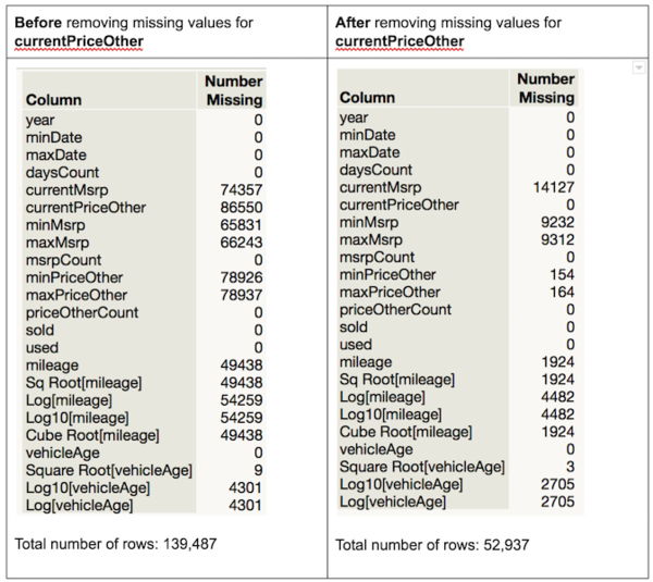
We chose to remove the rows which have missing values of ‘currentPriceOther’ since that is the target variable. Without data from the target variable, the row would be unable to be used in the model. After removing the rows with missing values of ‘currentPriceOther’, we can see that there is a significantly lower percentage of missing values.
Removing Outliers
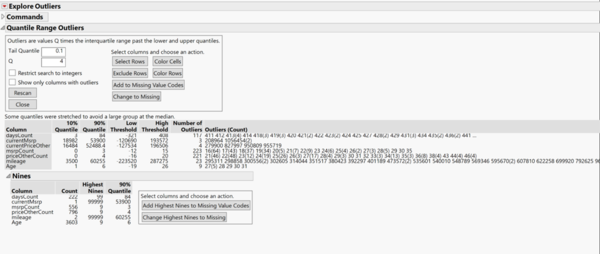
Outliers have extreme values that can largely influence our statistical analysis. While it may represent natural variation in our data, we decided to set the standard in classifying a data point as an outlier by using the Quantile Range Outliers in JMP. We chose Quantile Range Outliers instead of the other 3 possible choices such as Robust Fit Options, Multivariate Robust outliers and Multivariate k-Nearest Neighbor Outliers because the Quantile Range Outliers does not assume distribution associated with the data. Extreme values are calculated using the multiplier of the interquartile range(IQR).
We used a value of 0.1 for the Tail Quantile, and 4 for Q, which means in identifying the outliers, values have to be 4 times for than the IQR. All the values in the low threshold is negative,which means only the high threshold is considered as a qualifier.
| Variable | High Threshold | Max Value | No. of outliers | Explanation |
|---|---|---|---|---|
| daysCount | 408 | 522 | 117 | In building a pricing model, we are looking at used cars that have a reasonable days to market period. For these cars beyond more than a year, cases of such car existing could be due to:
Hence it may not be a relevant indicator for our pricing model. |
| currentMsrp | 193,572 | 1,056,454 | 3 | Blanket rule for a generalised model. |
| currentPriceOther | 196,506 | 955,719 | 4 | Blanket rule for a generalised model. |
| mileage | 287,275 | 962,525 | 23 | Cars driven beyond 200,000 miles are considered the high mileage for used cars. https://www.reference.com/vehicles/considered-high-mileage-car-e661f36f0817e76b |
We did not consider removing outliers for msrpCount, priceOtherCount and Age because these are calculated variables based on the initial variables in currentMsrp, currentPriceOther and for year variable, we are not removing the possibilities of vintage cars which can be manufactured in 1983.
Another advantage of Quantile Range Outliers is that it identifies the Nines. In most industries, a high value of 999999 is commonly used to fill in for a missing value. Though our analysis we found that the number of nines found in the dataset does not reflect that it has been used to recode for missing variables. The highest count was 3603, and it was found for Age, which reflects cars that have been produced in 2008. In addition, we consulted with the developers to how they have recoded missing values, where it is left as it is.
In conclusion, the total no. of outliers removed are insignificant compared to our dataset, hence we chose to remove the abovementioned outliers.
Is the dataset large enough?
One of the questions we are asking is if the dataset is large enough given the degrees of freedom that we play with.
In the scope of our project which aims to do predictive modelling mainly through regression and considering other modelling techniques such as randomForest decision trees, our sample size of 52,937 is large enough considering that this dataset is representative of the BMW cars in United States even after removing outliers and excluding missing values.
Feature Engineering
Feature engineering is the process of manipulating and combining features to arrive at more informative ones. The process in which the features were engineered is outlined below.
carCategory
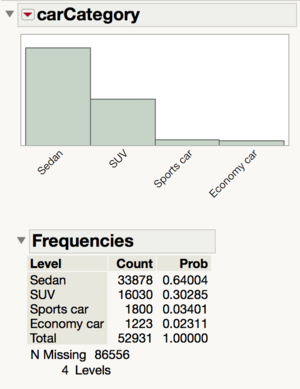
Due to the many car models in the column ‘cleanModelName’, we were unable to use a decision tree algorithm to classify the cars because there were too many categories. Therefore, we decide to reduce the number of categories to the following by creating a super group of ‘SUV’, ‘Sports car’, ‘MPV’, ‘Economy car’, ‘Sedan’. We also considered the type of vehicle in the column ‘vehicleType’, in the formula for the ‘carCategory’ column because some of the vehicles are motorbikes so we labeled them as ‘Motorbike’. The 10 missing values are null values.
vehicleType
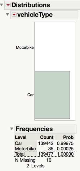
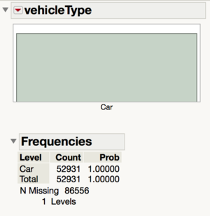
While cleaning the model names, we have also realized that some of the vehicles are not models of cars. Instead, they are models of motorbikes. As such, we decided to create a new column called ‘vehicleType’ to record whether each row contains a car or a motorbike. After excluding the missing values in ‘currentPriceOther’, we do not need this variable because the dataset now only contains cars.
Square Root[vehicleAge]
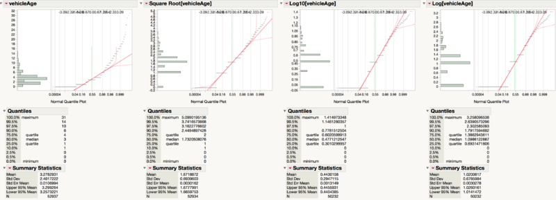
We understand that consumers would care about the age of the car because even if the models are of the same trim, it could be slightly different based on the year of production. After taking 2017 subtracted by the ‘year’ column, we are able to create a new feature which is the age of the vehicle. However, the age of the vehicle is not normally distributed so we performed a square root, ln and log10 transformation on it. A normal distribution is helpful later to increase the accuracy of our model. We then settled on using the square root transformation since according to the Q-Q plot, it is the closest to normality.
Concatenate[int,ext]
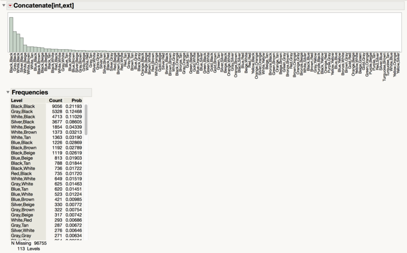
From our interactions with dealers, it seems that consumers care about the combination of colors of the interior and exterior. As such, it might be better to create a new categorical variable based on the combination of both the interior and exterior colors.
Sq Root[mileage]
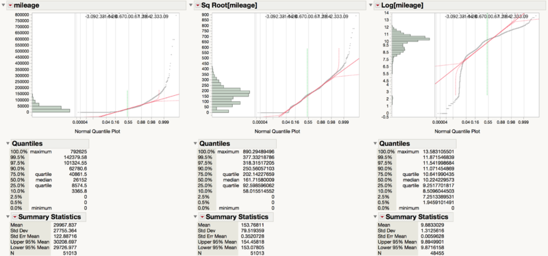
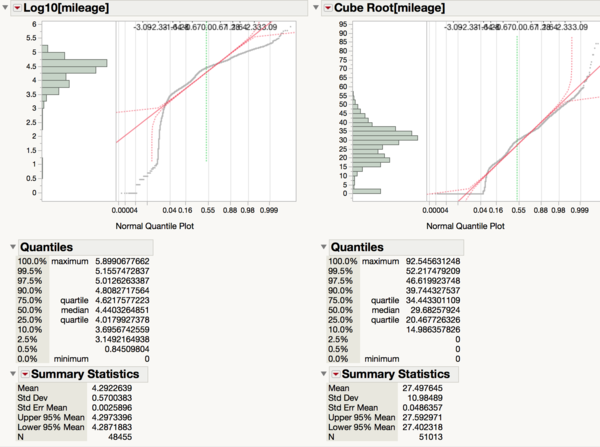
Since mileage is greatly skewed positively and there is high kurtosis, we needed to transform the variable to ensure that the variable is more normal. This will improve the accuracy of the regression later. After transforming it with square root, cube root, ln, and log10, we are able to see that the transformation that results in the most normal distribution is the square root one.
carCostCategory
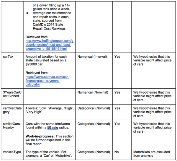
We hypothesized that the cost of car maintenance differs from each state and this will affect consumers preferences on used cars. Upon further investigation, we found out that there is a significant difference in terms of insurance cost, car tax between each state. Collectively, they affect the car cost by a large extent.
Using $25,000 as the cost of an average car in US, we are able to retrieve the cost of car maintenance for 3 years.
We then binned the variable to assign a categorical variable, carCostCategory, to each state which tells us how expensive it is to own a car compared to other states. There are 4 categories of car maintenance cost: Low ($8000 – $10000), Average ($10000 – $12000), High ($12000 – $14000), Very High ($14000 – $16000).
After creating a table of states which are binned into these 4 categories, we do an inner join with the primary data set which includes the used car sales data.
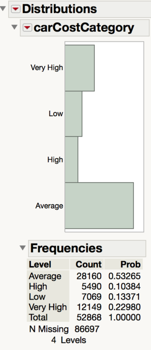
In the table above, we can see the frequency of used cars sold in states belonging in the 4 car maintenance categories.
Feature Selection
Feature engineering is fundamental to the application of machine learning. In order to obtain the possible features that might affect the pricing from the business perspective, we conducted surveys, phone calls and focus group discussions with dealers.
Primary Research
Our client, Automotive Ventures, gave us the contact of all dealerships in United States, which can be found in All dealers_Jully 11.xlsx . Out of the 30,000 dealerships we emailed for the survey, only 19 responded. The response rate was less than 1% and not all respondents completed the survey. Hence we turned to cold-calling dealers in Atlanta. However, there were only 2 successful calls. We managed to engage Hyundai Ford Legacy Dealership for a focus group discussion with 5 of their managers. We have also explored alternatives of viewing forums that Dealers usually go to, including DrivingSales.com, DealerElite and DealerRefresh.com to get any possible insights on dealerships.
Insights obtained: What factors affect their pricing decision making the most? In order of importance,
- Current inventory and competitor’s inventory – Dealers will price similar used cars according to the number of similar cars present in the market eg. if the dealership has 3 Ford SE SUV cars, and their competitor is bringing in 5 Ford SE SUV cars of comparable type, the dealer will be more inclined to lower their prices for the car.
- Seasonality – There are certain purchasing seasons for customers and wholesale customers which will result either in underpricing or overpricing their current inventory
- Industry news and trends, Competitive Intelligence reports are considered to be factors that are slightly important to a dealer’s decision making by influencing overall pricing strategy but may not impact in terms of effecting in the dealer changing price for a certain inventory.
Comments regarding predictive pricing models in the market
- “A lot of companies has to use 'price to market' and other factors can be market specific and industry trends are not always indicative of market or area trends” - Emanuel Jones, General Manager of Hyundai Sandy Springs
In identifying their competitors in the used car market, all dealers have consensually agreed that location (proximity) is the type of factor that they consider most. When asked how close a proximity is, they benchmarked within 10 miles to be their direct competitors and up to 100 miles as competitors. One of the dealer mentioned that customers are willing to travel across states to get a similar car that is priced $500 cheaper.
Customers are maker- sensitive, which means different makes attracts different profile of customers.
- “Hyundai customers are price sensitive. They are mainly shopping price and inventory. “ - Keith, Used Car Sales manager
For dealers, they try to justify pricing with the specifications that come along with the cars. Some customers may argue why the same car can have different price, and the dealer explains the specifications to make sure that the comparison is “apple to apple”.
With these insights obtained, below are the actions we tried to incorporate in our variable selection:
Defining a market for similar cars
- Pricing is affected by market forces of demand and supply. Hence we are creating another variable selection of “similar cars” which is calculated by identifying similar cars in terms of model and trim within 50 mile radius and excluding the similar cars inventory of the dealership.
- The variable “similarcars” will then be included in the modelling and regression analysis.
Seasonality
- There are effects of pricing seasonality and we asked the developers if the dataset stored in AWS S3 is complete. David Chisnell mentioned that as the dataset kept changing, the dataset that is stable and reliable only starts from September. Since we do not have a full year cycle of data, we are unable to analyse effects of seasonality on pricing.
Generalised model after filtering makeName of cars
- As mentioned by the dealers, the different make of cars attract different type of customers and are priced differently. In terms of creating the model, we decided that make should be a filter for the generalised model as customers are aware of the make of car that they would like to purchase.
Check for multicollinearity
To ensure that regression can be performed well, we would need to ensure that there is little multicollinearity between variables.
Multicollinearity is problematic because it can increase the variance of the regression coefficients, making them unstable and difficult to interpret.
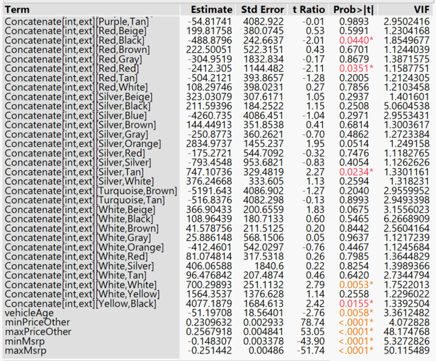
Variance inflation factors (VIF) measure how much the variance of the estimated regression coefficients are inflated as compared to when the predictor variables are not linearly related. As such, VIF is used to describe how much multicollinearity exists in a regression analysis. We used the least squares method to determine the VIF. A high VIF of more than 10 reveals high collinearity. Due to high multicollinearity, where VIF>10, we remove the columns maxMsrp and maxPriceOther.
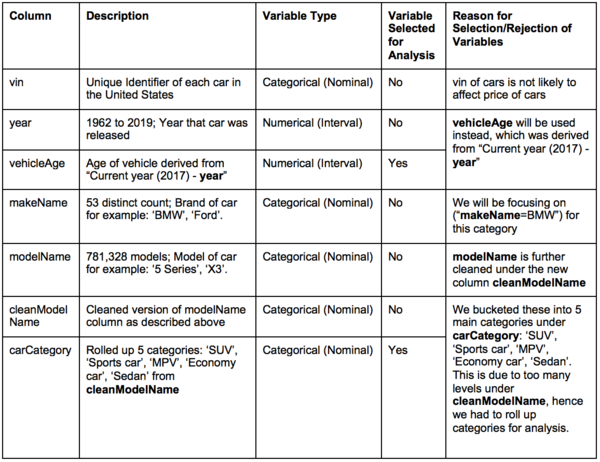
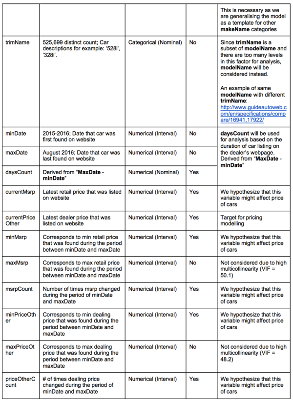
Selected Features
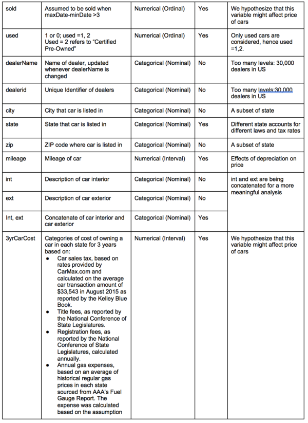
The variables shown in the above table contains two main types: numeric variables and categorical factor. Machine learning algorithms such as penalised regression or parametric tests analyse only numeric variables. The standard method for converting categorical variables to numeric is to code them into several new columns of attribute data. If an attribute has N possible values, it gets coded into N - 1 new columns of data as follows. Hence to include the categorical factors and its levels, we have recoded each level into a dummy variable for analysis.
