T15 Final Delivery
Dataset
Data Retrieval
The data used in this project is questionnaire result from the latest PISA survey in 2012. All raw data files are publicly available on PISA website (https://pisa2012.acer.edu.au/downloads.php). However, the raw data is in flat file text format, where a fix number of characters represent a value (eg. first 3 letters indicate country code), as follows:
The raw data in this form is not ready for cleaning and analysis. PISA database has scripts to convert the raw text data into table forms.
- Download raw questionnaire results (zipped text files) from PISA 2012 website and extract
- Retrieve SAS programs for appropriate data files
- Open the SAS scripts in SAS Enterprise Guide
- Ensure that the path to raw text files are correct
- Run the programs in SAS Enterprise Guide to get output SAS data table
- Export the output SAS data table in desired formats (.sas7bdat, .csv and so on); display labels as column names for easy interpretation later on.
Data Extraction
Only Singapore data is of interest for our scope of project, therefore only the records with Country code ‘SGP’ are extracted. This process gives us the following for analysis:
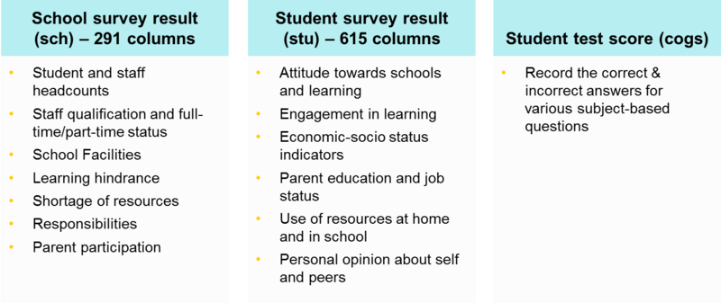
- School survey results - 172 secondary schools
- Student survey results - 5,546 records, approx. 35 students per school
- Student test score in Math, Science, Reading, Computer-based assessment
Each of the 3 mentioned data tables have a rich set of attributes. The summary below shows an overview of aspects that the data covers.
Data Preparation
The data preparation follows 3 basic steps.
Step 1: Aggregate student test score
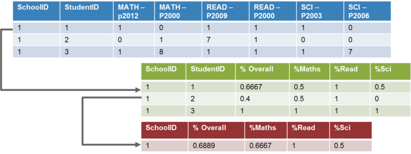
The original student test score table records the correct and incorrect answers by each student. We convert these into percentage score of each student by dividing the total number of correct answers by the total number of questions student attempted. Questions that are labeled 7 and 8 are not applicable to that student, and thus not taken into account when calculating percentage score.
Finally, we calculate the average test score for each school, in each subject based on student percentage score.
Step 2: Joining data tables
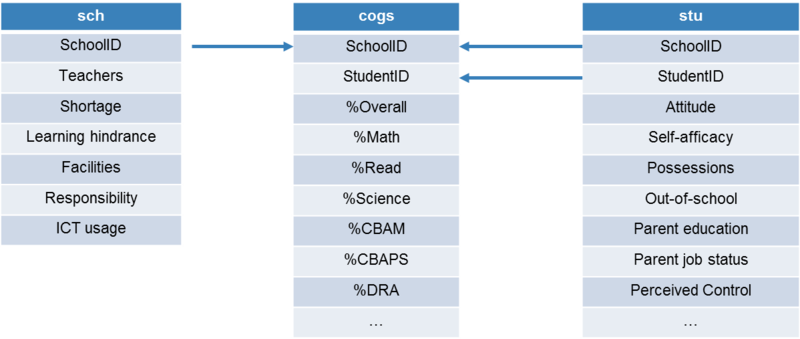
Score data and school data tables are joined by matching school ID. Since the granularity of these 2 tables is not the same – for score table, each record represents one student; for school table, each record represents one school – hence the need to aggregate data in score table in Step 1. The aggregated score will then be joined with school data table.
Joining score table and student table is more straightforward, simply by matching school ID and student ID. As the result of this step, student score will be used as measure for their academic performance, and other factors from school and student data tables will be used to help explain the difference in their performance.
Step 3: Data cleaning and standardization
Missing records in PISA data follow a consistent set of labels: ‘I’/’Invalid’, ‘M’/ ‘Missing’ and ‘N’/’No response’. In JMP Pro, we used Standardize Attribute to convert these values into a common null, so that JMP will recognize them all as missing data and process accordingly when building models.

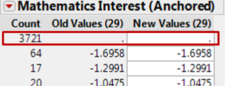
Upon checking for missing data pattern, some attributes are revealed to have more than 50% null values. These will be excluded from analysis. An example is given below: out of 5,546 records in student table, 3,721 records in Mathematics Interest (Anchored) are missing, so this attribute will not be chosen for analysis.
Lastly, attributes that do not help differentiating the entities in data are also excluded. For example, all attributes regarding “Acculturation” aspects only have ‘N’ values (No response) and these too will be excluded.
Methodology
Framework of analysis
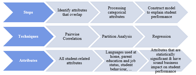
Understanding that student performance is affected by a school, family and personal factors, the analysis is carried out based on this assumption. At the school level, the steps to analyze data can be summarized as such:

The rationale of such a framework is to first have a good overview of school performance in Singapore, then slowly expanding the analysis to consider more factors as we formulate more in-depth business questions, based on an increasingly better understanding of the data and context. The framework is applied iteratively so as to refine the models.
In the first step, the goal is to have an overview of academic performance of schools in Singapore, hence distribution analysis is done using school test scores. Thereafter, having identified the spread of performance, we separate schools into different segments, based on their academic results, and study each of the segments to observe how school factors might differentiate their students’ performance. Features that separate high-performing from low-performing schools are to be identified, and we aim to profile the schools using those features. Finally, a regression model is constructed to explain in greater details to what extent the factors might cause student performance to change.
At the student level, the framework and techniques applied are largely the same as with schools. However, understanding that student data is more atomic and also has a richer set of attribute, we use score as the direct measure to build models, instead of segmenting students based on their performance as done with schools.
Techniques of analysis and variable selection
K-means clustering
K-means clustering is used to segment the schools based on their student performance. To this end, in JMP Pro, we perform Cluster analysis, with the average school scores in each subject as response variables. In terms of k-value, numbers 3-6 are chosen. This is due to the consideration that upon segmenting the schools, we will study the profile of each cluster and ultimately devise recommendation accordingly; hence clusters should come with a reasonably large number of data points, and that too many clusters are not favourable. The configuration in JMP Pro is shown as follow:
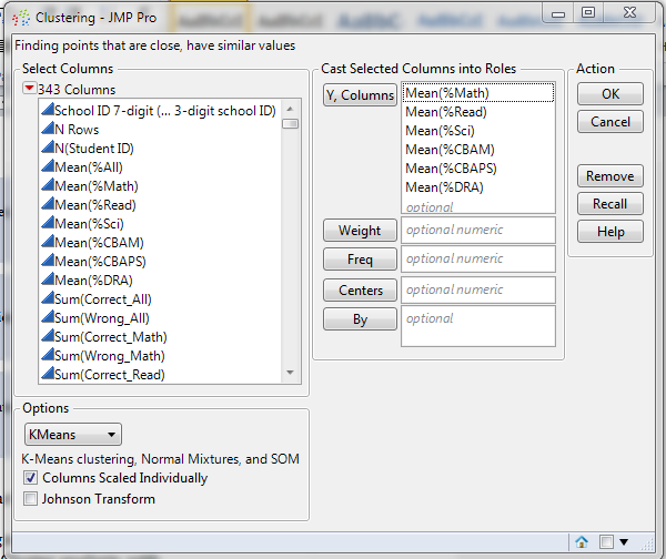
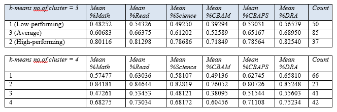
Running the analysis gives us the following clustering results:
Table 1: Results from k-means clustering

Statistically speaking, k = 4 gives the best result. However, eventually k = 3 is chosen for further analysis because, as shown below, when using 4 clusters, the lowest performing schools simply get further segmented but this does not give much additional insights. With k=3, we already achieve a clear segmentation and it makes logical sense to consider the schools as low-performing, average and high-performing.
Table 2: Results from k-means clustering (k=3 & k=4)
Partition analysis for school profiling
Using the clusters in the previous step as response variable, we use decision tree to profile the schools as below. This analysis will split the data according to school cluster, using the attribute that gives highest LogWorth, meaning that the attribute has the greatest impact in differentiating the schools.
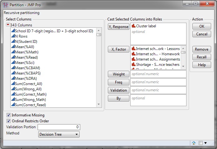
In order to observe the combined effect of all school factors on the student performance, we use 225 attributes, all of which have been checked for missing data (attributes with more than 50% missing data are excluded). Running the analysis results in a decision tree with RSquare value of 0.703 and total number of splits being 20. The details of this decision tree will be discussed in later section.
Table 3: Decision tree analysis results
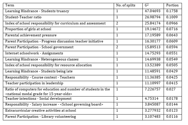
Using the tree, it is thus possible to identify the features that differentiate the schools into high-performing and low-performing clusters. The result will be discussed in the later sections.
Constructing regression model
Creating dummy variables for categorical attributes
For regression analysis to account for categorical attributes, they need to be converted into numeric form. Partition analysis can also be used to generate dummy variables for this purpose. Using school cluster (for school-level analysis) and student score (for student-level analysis) as response variables, Partition analysis will generate dummy variables for selected categorical attributes, such that the difference between nodes will be greatest.
School-level
There are several regression models to be built. For analyzing performance at school level, the following configuration is carried out in JMP
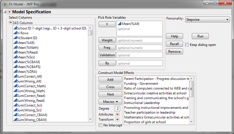
Response variable in this case is the overall mean score of each school, but we extend the analysis to cover all subject scores, which are Mathematics, Reading, Science and Computer-based assessment. The purpose is to compare the impact, if any, that various factors have on different subject performance by students. We will also be able to compare the extent of impact and how relatively important the factors.
The type of regression used is Stepwise, with p-value threshold as stopping rule. This allows us to interactively refine the regression model by adding/ removing attributes as necessary. Attributes selected to build regression model should have p-value (Prob>F) of 0.01 or less.
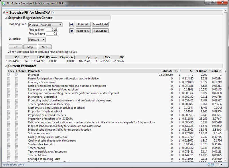
Student-level
At the student level of analysis, the subject scores are used as response variables, and the factors used to build regression models are numeric attributes and dummy variables of categorical attributes generated in the previous section. The stepwise configuration for student-level regression analysis is as follow:
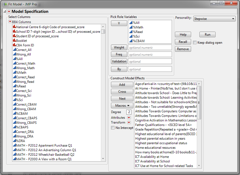
Similar to school-level of analysis, we use p-value threshold as the stopping rule. Variables selected to run models must have p-value (Prob>F) less than 0.01.
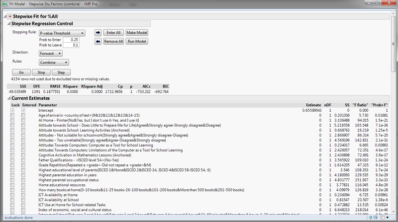
Using the standard techniques discussed above, we build on the student-level analysis by segregating students from low-performing schools from those from high-performing schools, and build separate regression models for each group. This is to discover more in-depth what constitutes the difference in performance for students on individual level, separate from the school factors. We have also noticed that some students from low-performing schools can still perform reasonably well; this group of students needs to be studied more carefully. Understanding how personal factors can overcome environment factors when environment is less than ideal could be the key to improving performances of students in Singapore.
School-level Findings
Exploratory Data Analysis
We conducted a distribution analysis and based on our findings, we created a tableau software visualization to enable users to analyze data from the school level and eventually deep dive into the performance of individual schools. In this section, we will discuss our findings.
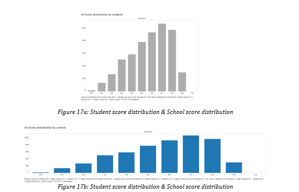
Majority of schools in Singapore are performing well academically, as seen in Figures 3a and 3b above, where the distribution of scores on both student and school levels are right-skewed.

However, we also found significant variation of performance amongst the schools. Figure 18 above shows a boxplot of the individual school performances. Although mostly right-skewed, the scores of students are widely distributed.

Performance of high-performing schools is seen to be high and consistent (Figure 19a above), ranging about 0.7 to 1.0. However, those of the low performing schools show a much greater disparity (Figure 19b), with scores ranging from 0.0 to 0.9. This suggests that not all schools are doing well and there is a significant disparity in school performance that requires further investigation.
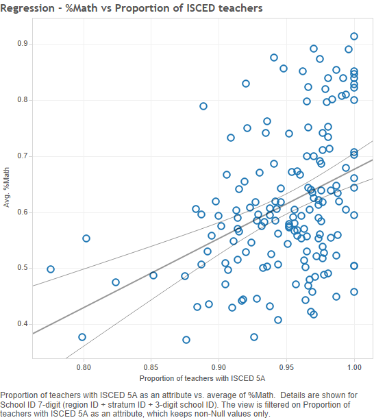
We can see that proportion of teachers is essential to the performance schools, especially in subjects like Mathematics. Figure 20 shows a relatively strong positive correlation between student performance in Mathematics and proportion of qualified teachers in schools.
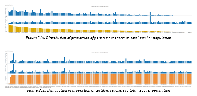
Figures 21a and 21b illustrate the proportionate staffing levels of part-time and full-teachers in schools. Not all schools have desirable staffing levels, with some having as much as 20% of their teachers working part-time.
Profiling high performance and low performance schools
Decision tree analysis

As addressed in previous section, based on the clusters, we conducted a decision tree analysis to identify the different profiles of the schools in each cluster. Figure 22 shows the split history with the resulting R-square of each split. Splitting can go up to 20 levels, but we decided on 15 splits, since there is marginal improvement in R-square beyond that point. We then used the tree to profile the characteristics of high performing and low performing schools.
Table 4: Column Contributions by partition analysis (Outcome = Cluster)
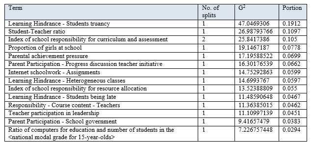
Table 4 above shows the top factors that differentiate between the low, average and high performing schools. Based on the results, quality of student attendance is the biggest differentiator of school performance as the distinction between the 2 clusters is biggest when it comes to truancy. Majority of good schools have zero cases of truancy and better ones have no cases of late attendance (Visual decision tree in Appendix A). This is consistent with studies that show better attendance is related to higher academic achievement for students of all backgrounds.

Figure 23 above highlights the characteristics and differences that define high and low performing schools. High performing schools have no incidence of truancy and take charge of their curriculum to cater to their unique circumstances, whereas low performing ones see a higher rate of truancy and pay less attention to their course curriculum. Parents of students in those schools are also less involved in their child’s learning process.
Multiple regression model
Numeric factors that affect test subject performance
Table 5: Multiple regression model using numeric factors (for overall score)
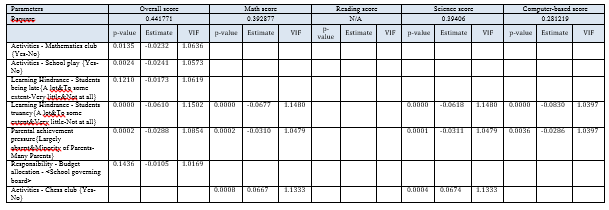
Using multiple regression model of the numeric factors, we identified the factors that affect the overall school test scores (See Table 5). The model shows a good fit with a R-square of about 0.404, covering 40.4% of the data given. The p-value is the probability of obtaining the estimated value of the parameter if the actual parameter is zero. The smaller the p value, the more significant the parameter is and the less likely it is that the actual parameter value is zero. As seen in Table 5, the p-value of all factors are below 0.05 and VIF is relatively small, indicating that all above factors are statistically significant with little collinearity between them. (Full results in Appendix B)
Looking at the estimates, we see a strong positive correlation between proportion of teachers with tertiary education and school test scores, indicating that quality teaching staff is key to good school performance. It is also important to ensure teacher morale is high, with its positive estimate of 0.031614.
Table 6: Significance of selected numeric attributes to school performance scores

This remains consistent when we extended the analysis to different subjects – Math, Science, Reading and Computer-based assessments – as seen in Table 6 above. For comparison, we looked to the log worth, p-value and estimates of each of the parameters to determine their importance across the subjects. While all factors affecting the overall score are significant for the individual subjects, some factors are more pertinent to specific subjects. For instance, having a good student-teacher ratio is important for reading scores and it is important for the schools to have control over their operations for students to do well in science and computer based assessments. Nevertheless, proportion of tertiary-educated teachers remains the top factor across the board and thus, having well-qualified teachers with high staff morale is really crucial for school performance.
Surprisingly, 27% of Singapore schools reported a shortage of teaching staff, especially for science teachers. And it is top amongst the all resource shortages reported by schools. However, as the data is highly aggregated and categorical– they only report the shortages in categories (e.g. “a lot”, “to some extent”, “very little” and “not at all”) – it is very difficult for us to examine the extent of the shortage if we are not able to quantify them. It is thus subjected to the school’s opinion and our analysis results would not be comparable.
Categorical factors that affect test subject performance
Table 7: Significance of selected categorical attributes to school performance scores
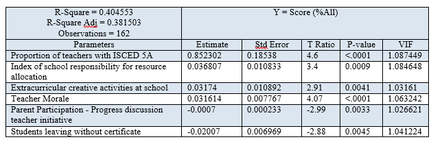
We also did the same for categorical attributes and Table 7 shows the most significant categorical factors that affect school performance. Student attendance remains the most significant factor, with student truancy being significant across the board and student lateness being significant to the overall test scores. Students also perform better when parents show concern for their child’s progress and give them the pressure to do well academically. Some school activities actually show to have a positive effect on results, related to Mathematics, chess and theatre. These activities allow children to engage in subject-related activities or activities that train their logic and strategic thinking.
Student-level Findings
Given that the multiple regression models for school level analysis only cover less than half (40.4%) of the dataset examined, looking at school environmental factors will not provide us with the complete picture. We will need to look into factors related to the family background and home environment of students to give more insights in explaining the differences in student performance.
Exploratory Data Analysis
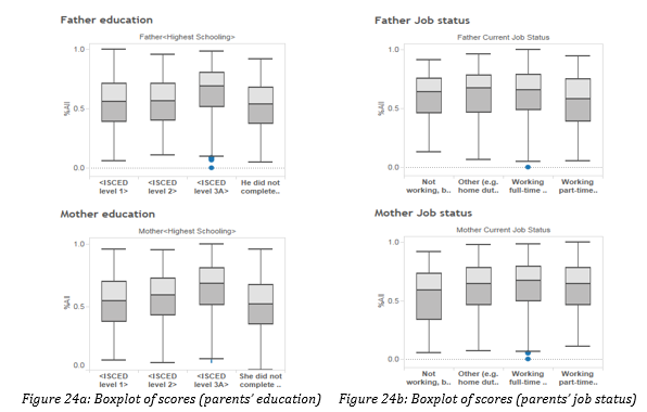
Results in Figures 24a and 24b show that parents’ education levels and employment status do impact student performance. From Figure 24a, we can see that students with parents that have at least an O level qualification tend to do better. Interestingly, those with parents working full time also tend to do better as seen from Figure 24b.
Multiple regression model
Variable selection
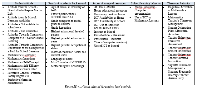
For our analysis, we considered a combination of family and personal factors in the following areas as seen in Figure 11, such as the student’s attitude towards school and learning, parents’ education and occupation, availability of educational resources, computer habits and subject-related activities engaged in and out of school.
Multiple regression
Table 8: Regression analysis results (selected)

Research shows that financial conditions will have a substantial impact on their academic achievement as those from poor families are likely to have adverse home environments which would affect their development. However, we observe from Table 8 that economic socio status of schools is actually insignificant to student’s test performance. This might be due to the nature of the survey. The PISA survey is designed for use on an international scale and since extreme poverty is largely absent in Singapore unlike other countries, the economic-socio index used might not be distinguishing enough for the purpose of our analysis. Nevertheless, results do show that having better access and appropriate usage of educational resources like books and computers will improve test performance.
Table 9: Regression analysis results (selected)
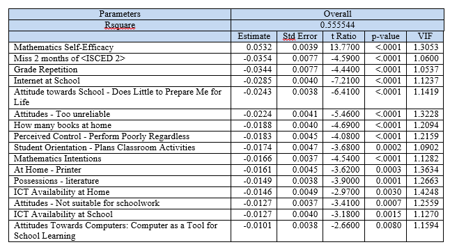
While material factors do have an influence on performance, students’ attitude towards school and learning is more crucial to their performance, as seen from Table 9 above. Personal attitude factors such as self-efficacy have a larger estimate as compared to home possession factors such as availability of books, printers and computers at home and in school. It is important for students to be confident in their abilities and believe in the usefulness of schools in preparing them for real life.
Factors that affect low performing schools
Table 10: Multiple regression results for student performance in high and low performing schools
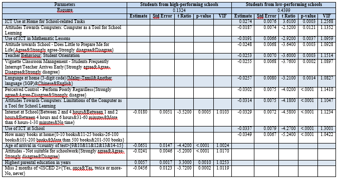
As the difference in student performance between low performing and high performing schools is significant (difference of 0.4 in their mean scores), factors that affect their scores may be different. Hence, we built separate multiple regression models for students in low and high performing schools to better identify factors that will truly affect their performance.
Table 10 shows the most significant factors identified through the regression analysis. All factors featured are statistically significant and there is little collinearity. Once again, we see that control over student usage of resources is important as an overuse of Internet at school will negatively affect the performance of all students, particularly those in low performing schools. Personal attitude and family background are more significant to student performance in low performing schools as compared to high performing ones.
Table 11: Most significant factors to student performance in low performing schools (descending order of significance)
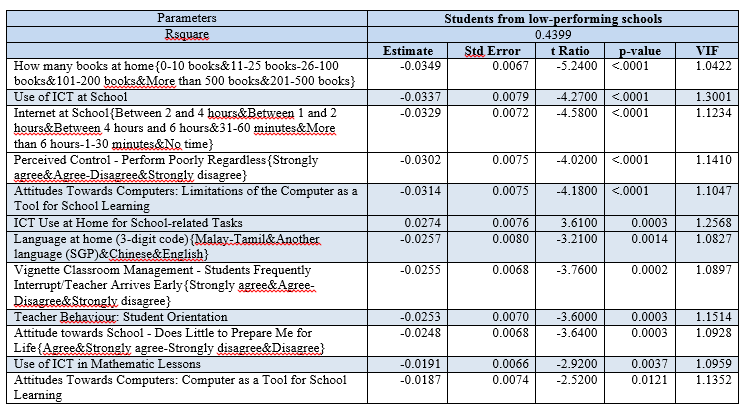
For low performing schools, it is important for students to have good access to resources, as seen from Table 11 where the availability of books and computers are parameters with the largest estimates with significant p-values. Use of computers in school and home to aid academic related tasks will help students score better.
Next would be the student’s personal attitude and mindset. Those that do well tend to have a strong internal locus of control, meaning they believe that their performance is primarily determined by through their own efforts. Those who believe that they will perform poorly regardless, tend to do worse. The effect of these personal factors exceeds the impact of classroom management, such as the amount of disruption in class and teachers’ efforts to engage students.
Discussion
General recommendation
Overall, all 3 aspects - school, family & personal factors - have a combined effect on the student and so a holistic view is required to improve student performance.
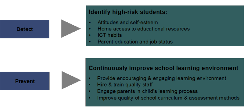
In general, based on our research, we recommend that for schools to take a 2-pronged approach to education and that is to detect and prevent. Research findings will be able to help schools better understand and identify high-risk students based on various factors such as their attitudes and self-esteem, access to educational resources, their computer habits and family background (Figure 12). This will strengthen the safety net in schools by allowing them to provide assistance as early as possible.
At the same time, it is important for schools to improve the overall environment by taking into account the factors seen in Figure 26.


