Difference between revisions of "Team Accuro Project Overview"
| Line 306: | Line 306: | ||
*Groups and outdoor seating have negative coefficients, possibly suggesting that more exclusive restaurants tend to have higher ratings. Typically, fine dining or up-scale restaurants are known to have these traits, and we hence hypothesize that this may well be the case here.<br> | *Groups and outdoor seating have negative coefficients, possibly suggesting that more exclusive restaurants tend to have higher ratings. Typically, fine dining or up-scale restaurants are known to have these traits, and we hence hypothesize that this may well be the case here.<br> | ||
| − | ==Testing Robustness== | + | ====Testing Robustness==== |
In order to test the robustness of our prediction formula, we performed the regression analysis on a training dataset which comprised of 60% of the dataset, with 20% allocated to training and test each. | In order to test the robustness of our prediction formula, we performed the regression analysis on a training dataset which comprised of 60% of the dataset, with 20% allocated to training and test each. | ||
[[File:Training validation test.png|center|Training, Validation, Test]] | [[File:Training validation test.png|center|Training, Validation, Test]] | ||
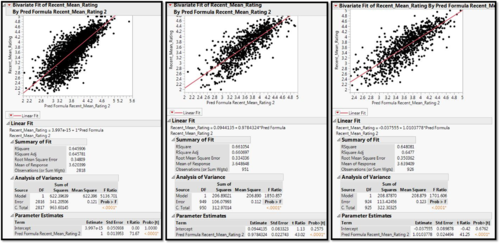
The results of the 3 runs are as follows:<br> | The results of the 3 runs are as follows:<br> | ||
| − | [[File:Results regression final.png|center|Regression results]] | + | [[File:Results regression final.png|500px|center|Regression results]] |
As we can see, the results have an R-square which is consistently around 65%, proving that the prediction formula is robust in calculating the results. | As we can see, the results have an R-square which is consistently around 65%, proving that the prediction formula is robust in calculating the results. | ||
Revision as of 11:12, 16 November 2015
Contents
- 1 Introduction and Background
- 2 Review of Similar Work
- 3 Motivation
- 4 Key guiding Questions
- 5 Project Scope and Methodology
- 6 Descriptive Analysis
- 7 Sentiment Analysis
- 8 Feature Extraction and Regression Analysis
- 9 Spatial Lag Analysis
- 10 Limitations and Assumptions
- 11 Deliverables
- 12 Work Scope
- 13 References
Introduction and Background
The Yelp Dataset Challenge provides data on ratings for several businesses across 4 countries and 10 cities to give students an opportunity to explore and apply analytics techniques to design a model that improves the pace and efficiency of Yelp’s recommendation systems. Using the dataset provided for existing businesses, we aim to identify the main attributes of a business that make it a high performer (highly rated) on Yelp. Since restaurants form a large chunk of the businesses reviewed on Yelp, we decided to build a model specifically to advice new restaurateurs on how to become their customers’ favourite food destination.
With Yelp’s increasing popularity in the United States, businesses are starting to care more and more about their ratings as “an extra half star rating causes restaurants to sell out 19 percentage points more frequently”. This profound effect of Yelp ratings on the success of a business makes our analysis even more crucial and relevant for new restaurant owners. Why do some businesses rank higher than others? Do customers give ratings purely based on food quality, does ambience triumph over service or do geographic locations of businesses affect the rating pattern of customers? Through our project we hope to analyse such questions and thereby be able to advice restaurant owners on what factors to look out for.
Review of Similar Work
The aim of the study is to aid businesses to compare performances (Yelp ratings) with other similar businesses based on location, category, and other relevant attributes.
The visualization focuses on three main parts:
a) Distribution of ratings: A bar chart showing the frequency of each star rating (1 through 5) for a single business.
b) Number of useful votes vs. star rating A scatter plot showing every review for a given business, with the x-position representing the “useful” votes received and y-position representing the for the business.
c) Ratings over time: This chart was the same as Chart 2, but with the date of the review on the x-axis
The final product is designed as an interactive display, allowing users to select a business of interest and indicate the radius in miles to filter the businesses for comparison. We will use this as a base and help expand on some of its shortcomings in terms of usability and UI. We will further supplement this with analysis of our own using other statistical methods to help derive meaning from the dataset.
2) Your Neighbors Affect Your Ratings: On Geographical Neighborhood Influence to Rating Prediction
This study focuses on the influence of geographical location on user ratings of a business assuming that a user’s rating is determined by both the intrinsic characteristics of the business as well as the extrinsic characteristics of its geographical neighbors.
The authors use two kinds of latent factors to model a business: one for its intrinsic characteristics and the other for its extrinsic characteristics (which encodes the neighborhood influence of this business to its geographical neighbors).
The study shows that by incorporating geographical neighborhood influences, much lower prediction error is achieved than the state-of-the-art models including Biased MF, SVD++, and Social MF. The prediction error is further reduced by incorporating influences from business category and review content.
We can look to extend our analysis by looking at geographical neighbourhood as an additional factor (that is not mentioned in the dataset) to reduce the variance observed in the data and improve the predictive power of the model.
3) Spatial and Social Frictions in the City: Evidence from Yelp
This paper highlights the effect of spatial and social frictions on consumer choices within New York City. Evidence from the paper suggests that factors such as travel time, difference in demographic features etc. tend to influence consumer choice when deciding what restaurant to go to.
Motivation
We believe that our topic of analysis is crucial for the following reasons:
1) It will make the redirection of customers to high quality restaurants much easier and more efficient.
2) It can encourage low quality restaurants to improve in response to insights about customer demand.
3) The rapid proliferation of users trusting online review sites and and incorporating them in their everyday lives makes this an important avenue for future research.
4) Prospective restaurant openers (or restaurant chain extenders) can intelligently decide the location based on the proximity factor to other restaurants around them.
Key guiding Questions
1) What constitutes the restaurant industry on Yelp?
2) What are the salient features of these inherent groupings?
3) How important is location within all of this?
4) What are some of the trends that have emerged recently?
5) Can we predict the ratings of new restaurants?
Project Scope and Methodology
Primary requirements
Step 1: Descriptive Analysis - Analysing Restaurants specifically for what differentiates High performers, low performers and Hit or Miss restaurants. For each of the 3 segments mentioned, the following analysis will be done:
- Clustering to analyse business profiles that characterize the market. Explore various algorithms and evaluate each of the algorithms to decide which works best for the dataset.
Step 2: Key factors identification for prescriptive analysis (feature selection) for new restaurants by region, in order to succeed. Regression will be used to identify the most important factors and the model will be validated so that we can analyse how good the model is. This will constitute the explanatory regression exercise.
Step 3: Spatial Lag regression model. This section will focus on Geospatial Analysis to examine the effect of location of a business on its rating. The goal of this will be to modify the regression model in Step 2 by adding the geospatial components as additional variables to the model. This section will explore the three spatial regression models and use the model that best fits the dataset:
- Checking for Spatial Autocorrelation: Spatial dependencies existence will be checked using Moran’s I (or any other spatial autocorrelation index) to see if they are significant.
- Weight Matrix Calibration: Developing the model will involve choosing the Neighbourhood Criteria and consequently developing an appropriate weight matrix to highlight the effect of the lag term in the equation.
- Appropriate model for Spatial dependencies: The Spatial Lag Regression Model and the Spatial Error Regression Models can both be used to understand the effect of location and whether the Dependent variable has dependence, or whether the Error Term does.
Step 4: Build a visualization tool for client for continual updates on business strategy. Focus will be to build a robust tool that helps the client recreate the same analysis on tableau.
Secondary requirements
A. Time series analysis of whether any major trends have emerged in restaurants by region – further decipher the does and don’ts for success
B. As an extension, we will also attempt to predict the rating for new restaurants, thereby informing existing restaurants of potential competition from new openings.
Future research
Evaluating the importance of review ratings for restaurants – Are they effective to improve ratings? Do restaurants that utilize recommended changes succeed?
Descriptive Analysis
Exploratory Data Analysis, Data Cleaning and Manipulation
We realized that the dataset actually contained records beyond the past 10 years. Since we did not want our model to be skewed by factors that were only important in the past, we chose to narrow down the dataset by only taking companies with greater than 5 reviews in the past 2 years (from 2013 to 2015), and changed the dataset to reflect that. Given that the mean rating was a rounded average for the ratings for all years, we had to compute the recent mean rating by combining the dataset containing reviews and filtering it by recent ratings, and subsequently mapping it back to the businesses dataset to develop a more recent and precise variable in mean ratings.
We suspected that it is likely for us to see a variance in the ratings and including that within our analysis would in fact allow us to see if highly rated restaurants get ratings high consistently. For that purpose, we again used the user review dataset and calculated the variance in rating for each business between 2013 and 2015 according to how users rated it.
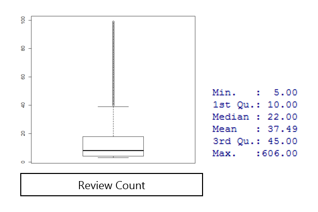
Review Count as a variable was also manipulated to reflect number of reviews for a particular restaurant between 2013 and 2015, and as mentioned above, only restaurants with greater than 5 reviews were included in the dataset.
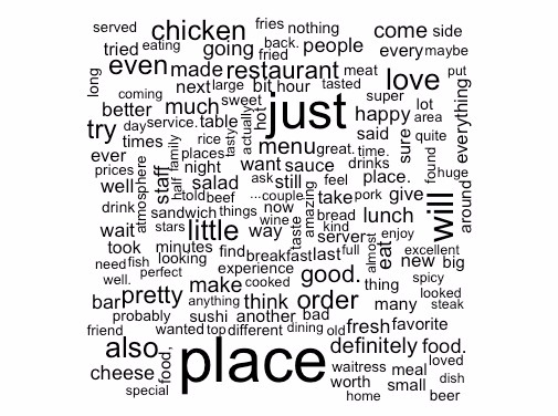
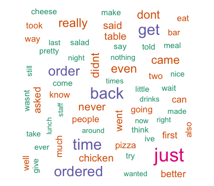
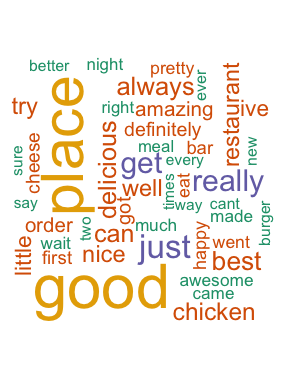
We also ventured into basic text analytics to analyse the review text for the restaurants on our dataset. Using R, we cleaned the review data and created word-clouds of reviews for all restaurants, high performing restaurants and low performing restaurants. This was done in order to gain an overview of the high frequency words associated with these restaurant categories. We generated three wordclouds.
Following are the most frequently used words for ALL the restaurants:
Following are the most frequently used words for low performing restaurants i.e. reviewers who gave a rating of 2 or below.
Following are the most frequently used words for high performing restaurants i.e. reviewers who gave a rating of 4 or above.
Given that there was a substantial number of missing values (>50%) for some of the variables, we decided that we needed to remove these variables.
Overall, we removed the 50 variables pertaining to Music, payments, hair types, BYOB, and other miscellaneous variables. Opening hour variables were computed into two new variables for Weekday opening hours and Weekend opening hours. As can be seen, many salient attributes that could contribute to how customers view the restaurant have been removed from the analysis due to bad data quality.
Since most of the fields consisted of binary data and still did not have all the fields, we decided that replacing missing values was essential for clustering and regression analysis. Therefore we proceeded with imputing missing values with the average score for each category. Since binary variables were changed to continuous data, we essentially took the average and imputed the values as such.
Restaurants were tagged under a string variable called “Categories”. This variable consisted of tags for a particular business and consisted of fields like “Greek”, “Pizzas”, “Bars”, etc. We found that these categories might be useful in determining the level of success of failure for restaurants. Unfortunately, since we had 192 different categories, we grouped categories according to high performing ones and low performing ones, and created two numerical variables titled “high performing categories” and “low performing categories”. This will hopefully lend greater credibility to the level of analysis and provide a better explanation for the performance of restaurants.
Clustering
a) For K-means and K-Medoids Clustering, all variables must be in numeric form. Therefore, the following changes were made to the different variable types to convert them to numeric form.
b) For Mixed Clustering, no data conversions were required as the algorithm recognises all types of data. Missing values are also acceptable.
However, due to lack of meaningfulness of some variables in the clustering process, such as name, business id, the variables were assigned a weight of 0 to exclude them from analysis.
K-Means Clustering
After converting all variables into numeric form and imputing the missing values with average value, k-means clustering technique was used to cluster the businesses.
However, due to the nature of the data, k-means clustering is not be the most ideal clustering algorithm. The issues with the technique are as follows:
a) As binary variables were converted into numeric, the resulting clustering means may not be as representative.
b) Due to presence of outliers in the data, the clustering will be skewed.
K-Medoids Clustering
After converting all variables into numeric form and imputing the missing values with average value, k-medoids clustering technique was used to cluster the businesses.
K-Medoids clustering is a variation of k-means clustering. In K-Medoids clustering, the cluster centres (or “medoids”) are actual points in the dataset. The algorithm begins in a similar way ask-means by assigning random cluster centres. But, in k-medoids the cluster centres are actual data points. A total cost is calculated by using the summing up the following function for all non_medoid-medoid pairs:
cost(x,c)=∑_(i=1)^d(|xi-ci|)
, where x is any non-medoid data point and c is a medoid data point.
In each iteration, medoids within each cluster are swapped with a non-medoid data point in the same cluster. If the overall cost is less (usually defined by Manhattan distance), the swapped non-medoid is declared as new medoid of the cluster.
Although, k-medoids does protect the clustering process from skewing caused by outliers, it still has other disadvantages. The issues with the K-Medoid technique are:
a) As binary variables were converted into numeric, the resulting clustering means may not be as representative.
b) The computational complexity is large.
Mixed Clustering
Partitioning around medoids (PAM) with Gower Dissimilarity Matrix
As our dataset is a combination of different types of variables. Therefore, a more robust clustering process is needed which does not require the variables to be converted to numeric form.
Gower dissimilarity technique is able to handle mixed data types within a cluster. It identifies different variable types and uses different algorithms to define dissimilarities between data points for each variable type.
For dichotomous and categorical variables, if the values for two data points are same, dissimilarity is 0 and vice versa.
For numerical variables, distance is calculated using the following formula:
1- sijk = |xi – xj|/Rk
where sijk is the similarity between data points xi and xj in the context of variable k, and Rk is the range of values in variable k
The daisy() function in the cluster library in R is used for the above steps.
The dissimilarity matrix generated is used to cluster with k-medoids (or PAM) as described earlier. The dissimilarity matrix obtained serves as the new cost function for k-medoids clustering.
We call this two-step process “Mixed Clustering”. This method has a number of datasets:
a) As k-medoids method is used, the clustering is not affected by outliers.
b) Clustering can be done without changing the data types.
c) Missing data can also be handled by the Gower dissimilarity algorithm.
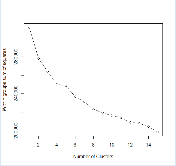
Elbow Plots:
The following elbow plot was generated using R.
As there is a clear break at 4 number of clusters, we proceeded to carry out clustering with 4 clusters.
Mixed Clustering:
Published Tableau page
Sentiment Analysis
Motivation
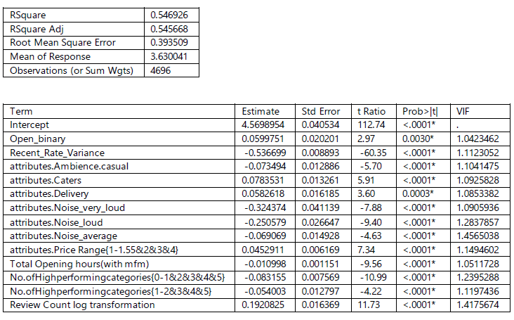
Upon preliminary regression analysis, we found the following results:
We felt that the Adjusted R square could be improved. Furthermore, we did not consider the content of a review within this calculation. We therefore wanted to include some of the salient features of that make up a review. To do this, we decided to undertake basic sentiment analysis.
Approach
There are various methods that can be used for Sentiment analysis. The following Wikipedia link provides a good summary for the same:
https://en.wikipedia.org/wiki/Sentiment_analysis
While Keyword spotting was initially a good enough heuristic choice, we sought to expand further from there.
Among the competing methods used, we therefore chose the Lexical Affinity model. Specifically, we sought to compute a polarity variable for each review provided for the business. As before, a subset of reviews was chosen (for restaurants in Arizona and reviews between 2013 to 2015).
In order to incrementally build on this lexical prediction, we chose a simple polarity as our first step by looking at the difference of positive words and negative words. It was important to choose the right method in selecting the positive and negative words, so we utilized the library developed in widely cited papers on the lexical method. The library for positive and negative words can be found here:
File:Positive words.txt
File:Negative words.txt
As can be seen, the number of positive words is around 2006, with negative words being around 4783. These lists also include commonly misspelled words in opinions that can be associated with opinion based reviews in past research papers. The two files above cite the source of these words as well.
The results of the additional variable were as follows:
- Mean Sentiment - 4.15
- Variance in sentiment - 22.02
- Correlation with Mean Average Rating - 0.58
Limitations
There are number of limitations to the aforementioned approach. For instance, this approach does not include negaters, amplifiers and decreasers that inflate, reverse or deflate the emotion in an opinion. This means that the final solution tends to not be as robust as it could be.
Furthermore, this analysis does not include sarcasm and emoticons in the analysis to convey emotion, making the analysis limited in being able to show the rating.
Another limitation is that we have not included any topic extraction from the reviews. If the sentiments could somehow be linked to components of a business, the salient features of that business could be extracted. For example, if a business is rated 2 and its service is consistently criticized, it could be a major source of analysis in explaining the variation between this business and another business rated as 2.5.
Future Work
Continiung on from the Limitations, this analysis should basically look to address all of the limitations as mentioned above. Furthermore, future research must also include the variety of mixed models developed by researchers in several academic papers to predict ratings of restaurants, so that more of the variance is explained.
Feature Extraction and Regression Analysis
Approach
Step 1: Stepwise Regression
Due to over 50 variables being part of our dataset, we realized that simply doing a regression may not yield the most representative results. Furthermore, the models may be over-fitted and may hence cause problems when predicting ratings for the entire dataset.
Therefore we started with Stepwise Regression. Stepwise regression is a semi-automated process of building a model by successively adding or removing variables based solely on a certain criteria of their estimated coefficients. There are various techniques that set the criteria to do the same:
- Forward selection, which involves starting with no variables in the model, testing the addition of each variable using a chosen model comparison criterion, adding the variable (if any) that improves the model the most, and repeating this process until none improves the model.
- Backward elimination, which involves starting with all candidate variables, testing the deletion of each variable using a chosen model comparison criterion, deleting the variable (if any) that improves the model the most by being deleted, and repeating this process until no further improvement is possible.
- Bidirectional elimination, a combination of the above, testing at each step for variables to be included or excluded.
We chose to use Forward selection for our model because we had a very large set of variables and we wanted to extract just a few. Our general reasoning is essentially because we are on a fishing trip to find the best variables. In terms of criteria, we chose AIC.
Since we knew that this was not going to be our final model, we did not spend a lot of time delving into other stepwise techniques and picking the best one.
Step 2: Multiple Regression
The next step is to use Multiple Regression to test the significance of the variables which came as an output for Stepwise Regression.
When we first saw the results, we realized that some of the coefficients were not significant. This is understandable since Stepwise regression tends to be prone to overfitting. We iteratively removed the variables that were insignificant to finally arrive at the final results for each of the clusters identified.
Findings
Iteration 1: Interim findings
We understood that a lot of great insights can be derived from the model. We chose to highlight the most important ones below:
- Fit of Model is not that great for each cluster
- Adjusted R ranges from 0.19 to 0.46 – very little of the variation in the mean rating is explained.
- Quality of food or location could be a big factor affecting ratings
- Good for Dessert, Good for Late Night and more expensive restaurants indicates probably that fine dining restaurants tend to do well on Yelp
- Need to be mindful of noise levels, they play a big factor
Iteration 2: Final findings
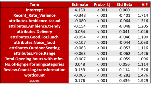
After including the wordcount and sentiment score as two additional variables in the equation, the results changed quite significantly:
- Adjusted R-square increases from 54% to 65% by virtue of including wordcount and sentiment scores into the model. This is a dramatic increase and expected since the sentiment plays a big part in explaining the ratings offered to a business. This is further substantiated where a high correlation of the sentiment score (r = 0.58) is observed with Recent Mean Ratings.
- The lesser the variance, the better your score. This basically indicates that good restaurants have consistently good reviews, owing possibly to consistency in service or network effect of users in affecting the perception of other users when they visit the restaurant. Either way, if you're in the good books, you'll tend to stay there.
- Groups and outdoor seating have negative coefficients, possibly suggesting that more exclusive restaurants tend to have higher ratings. Typically, fine dining or up-scale restaurants are known to have these traits, and we hence hypothesize that this may well be the case here.
Testing Robustness
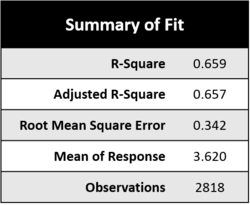
In order to test the robustness of our prediction formula, we performed the regression analysis on a training dataset which comprised of 60% of the dataset, with 20% allocated to training and test each.
The results of the 3 runs are as follows:
As we can see, the results have an R-square which is consistently around 65%, proving that the prediction formula is robust in calculating the results.
Assumptions
In analysing the results of the regression, we needed to check the assumptions that we made along the way and whether, in fact, they held true at the end of the regression. This would help us moderate our findings so that we don’t overstate the robustness of the results derived. The assumptions of a multiple linear regression are as follows:
1) Linear relationship and additivity
2) Multivariate Normality
3) No or little multicollinearity
4) No auto-correlation
5) Homoscedasticity
Spatial Lag Analysis
Approach
We believe that neighbourhood and location have a role to play in the overall star ratings of a restaurant in the Yelp dataset. This is why our group has forayed into exploring the spatial lag model for our project. ‘Tobler’s first law of geography encapsulates this situation: ‘‘everything is related to everything else, but near things are more related than distant things.’’ In context of our project, we suspect that the average rating of a neighbourhood affects the star rating of any restaurant within that area.
Step 1: Set Neighbourhood criteria
Deciding the neighbourhood criteria is critical for building the weights matrix. We have chosen Distance as our criteria which takes distance between two data points as a relative measure of proximity between neighbours. So the Weights Matrix is populated by values in terms of miles or kilometres or any other unit of distance. On the other hand, the contiguity criteria divides the data points into blocks and creates binary values for the weights matrix with 1 referring to 'neighbours' sharing a common boundary (adjacency factor) and 0 referring to distant businesses or 'not neighbours'. The third criteria is a more complex version of the first two which must only be set if the first two do not work.
Once the criteria has been decided based on the needs of the dataset we move on to the next step.
Step 2: Create Weights Matrix
The Weights Matrix summarises the relationship between n spatial units. Each spatial weight Wij represents the "spatial influence" of unit j on unit i. In our case the row and columns of our square matrix will have each unit on the two axis as being a restaurant with the diagonal being zero. Once the matrix has been created, it needs to be row standardised. Row standardisation is used to create proportional weights in cases where businesses have an unequal number of neighbours. It involves dividing each cell unit in a row by the sum of all neighbour weights (all values in that row) for that business.
Step 3: Check Spatial Autocorrelation
Next step involves checking the need for a spatial model. When do we decide that a Linear regression is not enough to predict our ratings and that our dependent variables may be spatially lagged? We use the Moran's Index or Geary's C to make this decision. The index of spatial autocorrelation we use is Moran's I which involves the computation of cross-products of mean-adjusted values that are geographic neighbours (i.e.,covariation), that ranges from roughly (–1, –0.5) to nearly 0 for negative, and nearly 0 to approximately 1 for positive, spatial autocorrelation, with an expected value of –1/(n – 1) for zero spatial autocorrelation, where n denotes the number of units.
We used R (function daisy) to compute the index (= 0.9409) which turns out to be significant for our model. Thus we can conclude that there is some spatial interaction going on in the data.
Step 4: Choose the appropriate Model
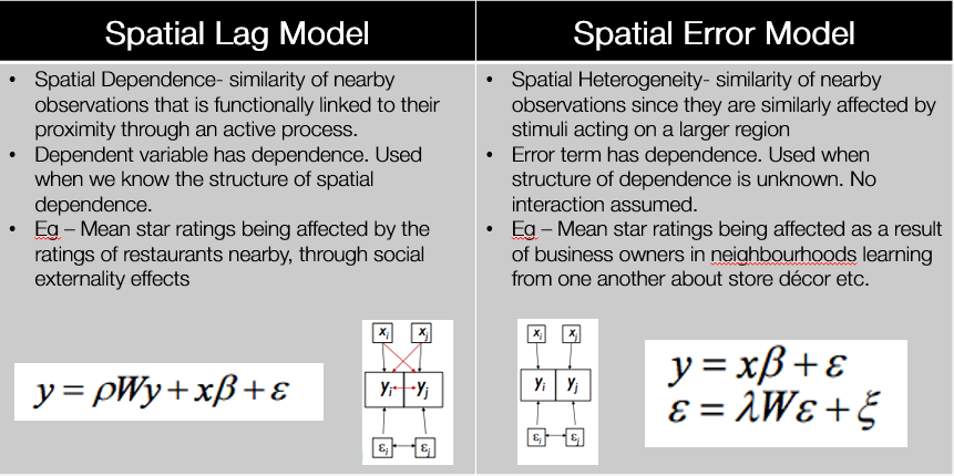
Now that we know for sure that we have strong spatial autocorrelation we must choose an appropriate model to explain it. The table below summarises the main differences between the Spatial Lag and Spatial Error Model. The Lagrange Multiplier Test is used to mathematically compute the significance of using each model. So far, we suspect that the Spatial Lag Model will be more relevant for our project.
Step 5: Build Spatial Regression Model
The final and conclusive step would be to build the Spatial Regression model which incorporates a spatial dependence. This is done by addng a 'spatially lagged' dependent variable on the right hand side of the regression equation. The model now looks like this: y= ρWy + xβ + ε (1-ρW)y= xβ + ε
where y= restaurant rating ρ= spatial correlation parameter W= Spatial weights x= other attributes β= coefficient of correlation ε = error term
Spatial Autocorrelation
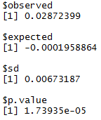
The output for Moran's I test using the distance criteria 1/d (inverse of distance in km) to construct the weights matrix can be seen below. Since the number for Moran's I is close to zero (0.028), this suggests that there is almost no spatial autocorrelation in our dataset. In order to further explore our results, we changed the criteria for the distance matrix several times in order to check for spatial dependencies. Following are some of the criteria used:
- inverse of distance squared
- inverse of distance raised to the power of 6
- contiguity matrix
Despite changing the weights criteria, Moran's index only increased marginally. Essentially, this meant that the star ratings of Yelp restaurants were spatially independent of their neighbour's ratings. To completely rule out any chances of spatial interaction we tested for correlation in other measures like count of ratings, ratio of high/low ratings, variance of ratings. As expected, once again, there was no spatial dependence.
Conclusion:
Due to the low value of Moran's Index for the different depenedent variables we contructed the model for, we can conclude that our dataset has no spatially correlated data-points i.e. Geographical location in terms of proximity with certain neighbours does not play much of a role in star ratings of restaurants.
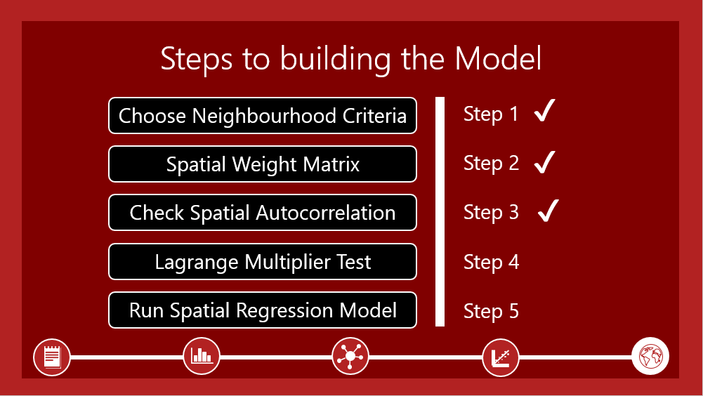
In summary, the steps achieved for the Spatial Lag model are as follows:
Limitations and Assumptions
| Limitations | Assumptions |
| Limited data points on businesses and cities | Project methodology will be scalable for looking at regional trends |
| Limited action-ability of insights since companies may not care about Yelp ratings | Project findings will help set priorities for improvement for business owners |
| Businesses attribute may not be completely accurate | Assuming that data has been updated as accurately as possible |
| Defining business categories | Assuming business tags under categories are comprehensive for the competitive set |
Deliverables
- Project Proposal
- Mid-term presentation
- Mid-term report
- Final presentation
- Final report
- Project poster
- Project Wiki
- Visualization tool on Tableau
Work Scope
Through this project we are hoping to build to an interactive dashboard as a solution to the ratings and recommendations system Dataset Challenge by Yelp. This will be in addition to the insights developed from statistical and machine learning techniques that can support decision making for businesses. Some areas of research we are looking into are:
- Cultural Trends
- Seasonal Trends
- Spatial Lag Regression Analysis
- Time Series Analysis
- K-Means, K-Medoids and Gower's Method for Clustering
- Explanatory Regression analysis

