Difference between revisions of "ANLY482 AY2016-17 T1 Group4: Project Findings"
| Line 142: | Line 142: | ||
===Clustering Analysis=== | ===Clustering Analysis=== | ||
| + | |||
| + | ====Rationale==== | ||
| + | |||
| + | Initially, K-means clustering in SAS Enterprise Guide was considered, but this procedure can only analyse numerical variables. The exploratory data analysis revealed that there were some important categorical variables such as marital status or nationality which is extremely essential in understanding the customer. On a side not, converting categorical variables to numerical variables is not a logical solution as it’s meaningless to calculate the Euclidean distance between the values of a categorical variable. | ||
| + | |||
| + | <br> | ||
| + | |||
| + | Hierarchical Clustering was avoided as it has higher complexity than the other clustering methods, thus it would take an extremely long time to experiment and execute an optimal clustering solutions for such a large dataset (consisting of nearly 140,000 customers). The complexity of hierarchical clustering is nearly O(), as opposed to O() for k-means clustering (Inaba, M.; Katoh, N.; Imai, H., 1994). But more importantly, there was no inherent hierarchy present in the data structure itself to use hierarchical clustering. | ||
| + | |||
| + | <br> | ||
| + | |||
| + | Thus, ultimately a Mixed cluster analysis was used to perform a clustering analysis on both categorical and continuous variables. Mixed cluster analysis extends the concept of Latent Class Clustering to a wide range of variables such as interval, nominal and date-time. SAS Enterprise Miner was used to execute the Mixed cluster analysis for the dataset. | ||
| + | |||
| + | ====Data & Methodology==== | ||
| + | |||
| + | The data preparation process was closely linked to the data analysis process. As opposed to the market basket analysis, a clustering analysis is usually analysed from the perspective of the customer. Thus the combined dataset was converted to a single customer view (SCV) where every row of the data represented one unique customer. The dataset consisted of demographic variables such as gender, marital status, age, and occupation. But along with demographic parameters, certain product variables were also computed to shed light on a customer’s behavioural parameters i.e. a customer’s knowledge, attitude and usage of the product. | ||
| + | |||
| + | Thus for the behavioural variables, the single customer view was linked to the contract header dataset and 4 variables were computed: total policies of a customer, total number of riders, total premium paid by the customer, total single premium paid upfront by a customer. The following Process Flow Diagram was used to import the data into Enterprise Miner: | ||
| + | |||
| + | [[File: riders.png | 700px |thumb|none|Rider Uptake Over Time]] | ||
| + | |||
| + | The clustering is automatically based to be computed on non-missing inputs, but this procedure leads to a loss of data and information. Thus an Impute Node was used to deal with missing values. In the property panel, the Default Input Method for both interval and class variables is changed to Tree. Thus this Impute node uses a tree method to replace missing values. | ||
| + | |||
| + | |||
<!--Body End--> | <!--Body End--> | ||
Revision as of 15:34, 2 December 2016
Contents
Mid-Term Findings
Exploratory Data Analysis
For our exploratory data analysis, we went with analyzing the three different aspects of the data, namely, the clients and the policies.
Distribution By Age
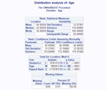
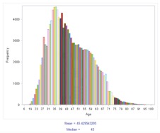
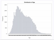
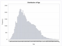
In the dataset, age was not a present field, so it had to be derived using the customers' date of birth. The current year was subtracted by the customer's birth year in order to generate a derived field, which was then the customer's age. Using SAS EG's 'one way frequency' feature, we were able to generate the age distribution for the clients.
From the data, we are able to see that the median age is around 45, with the standard deviation being around 13 years. However, there are missing age values, and those entries consist of 9% of the data, and have been excluded from this analysis.
We can also see that most of the customers are around the ages of 31 to 45, from the graph. It can also be observed that the graph is right skewed, because of this particular distribution
Distribution By Gender
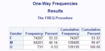
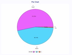
Clients were also grouped into their respective genders, and the distribution was then plotted into a pie chart. The males are denoted by the blue segment, while the females are denoted by the pink segment. Those clients that failed to disclose their gender, which appeared the dataset as "U", are denoted by the orange segment.
From the data, we are able to observe that around 53% of the valid clients are male, while around 46% are female. There is a very small percentage of individuals, however that did not disclose their gender (0.53%).
Distribution By Age & Gender
Below are two separate age distribution graphs that are grouped by gender. The graph on the top is for females while the graph on the bottom is for males. The bars are the frequency of clients who fall under that particular age.
For Females:
For Males:
What we can observe is slightly more women than men for clients aged 50 years old to their late 60s. However, we are also able to see that there are slightly more men than women clients for clients in their late 30s, by comparing both peaks, which both happen to fall within the similar age range of 30 to 45 years old.
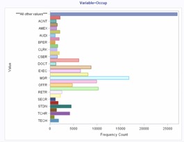
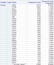
Distribution of Customers By Occupation
From the above analysis, we are able to observe that the highest group of customers are managers, followed by “OTHR”. This could possibly consist of other businessmen such as Entrepreneurs. Following that are a group that did not disclose their occupation. Engineers, Housewives and Executives follow after that.
Understand Policy Based Data
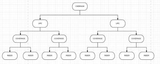
For policy based data, we would be looking at a few fields, namely, CHDRNUM, which indicates the unique policy number, RIDER, which indicates the rider index number, INSTPREM, which is the premium that has been paid up for that particular. Also, we would be looking at the columns LIFE and COVERAGE, which are the columns that define the index of each contract’s coverage. Essentially, this is the visual representation of how each contract is modelled:
Each CHDRNUM has many LIFE, which has many COVERAGE, which has many RIDERs. To illustrate, the table below shows a small sample of the data:
As seen from the small sample above, we can see that for a contract with CHDRNUM of 00240907, it contains two LIFE coverages, 01 and 02. Within each LIFE, COVERAGE then denotes each coverage plan within each Life Coverage. For each coverage plan, there exists various riders. However, one thing to take note of is that the all life coverages that come after 01 will be nested under the original coverage defined in the row where LIFE =01, COVERAGE = 01 and RIDER = 00. Therefore, if the product defined for the row of LIFE =01, COVERAGE = 01, RIDER = 00 is “Legacy Plan”, then the basic plan for the entire contract of 00240907 would be “Legacy Plan”. Also, another thing to take note is that as long as LIFE is not 01, then that particular record is a rider for the basic plan defined by LIFE =01, COVERAGE = 01, RIDER = 00 in that particular contract.
Policy's Uptake Vs Time
We plotted graphs for each of the basic plans and also for the riders, to allow the client company to understand the uptake of each basic plan over the years. The variable used in this analysis was the start date of the client's policy, and this was grouped by each unique policy, to generate one chart per policy.
For Basic Plans Only:
From this, they will be able to understand which plans have an increasing uptake rate, and which plans have a decreasing uptake rate. These graphs have been put into a separate PDF, for their perusal.
For Riders Only:
Finals Findings
Clustering Analysis
Rationale
Initially, K-means clustering in SAS Enterprise Guide was considered, but this procedure can only analyse numerical variables. The exploratory data analysis revealed that there were some important categorical variables such as marital status or nationality which is extremely essential in understanding the customer. On a side not, converting categorical variables to numerical variables is not a logical solution as it’s meaningless to calculate the Euclidean distance between the values of a categorical variable.
Hierarchical Clustering was avoided as it has higher complexity than the other clustering methods, thus it would take an extremely long time to experiment and execute an optimal clustering solutions for such a large dataset (consisting of nearly 140,000 customers). The complexity of hierarchical clustering is nearly O(), as opposed to O() for k-means clustering (Inaba, M.; Katoh, N.; Imai, H., 1994). But more importantly, there was no inherent hierarchy present in the data structure itself to use hierarchical clustering.
Thus, ultimately a Mixed cluster analysis was used to perform a clustering analysis on both categorical and continuous variables. Mixed cluster analysis extends the concept of Latent Class Clustering to a wide range of variables such as interval, nominal and date-time. SAS Enterprise Miner was used to execute the Mixed cluster analysis for the dataset.
Data & Methodology
The data preparation process was closely linked to the data analysis process. As opposed to the market basket analysis, a clustering analysis is usually analysed from the perspective of the customer. Thus the combined dataset was converted to a single customer view (SCV) where every row of the data represented one unique customer. The dataset consisted of demographic variables such as gender, marital status, age, and occupation. But along with demographic parameters, certain product variables were also computed to shed light on a customer’s behavioural parameters i.e. a customer’s knowledge, attitude and usage of the product.
Thus for the behavioural variables, the single customer view was linked to the contract header dataset and 4 variables were computed: total policies of a customer, total number of riders, total premium paid by the customer, total single premium paid upfront by a customer. The following Process Flow Diagram was used to import the data into Enterprise Miner:
The clustering is automatically based to be computed on non-missing inputs, but this procedure leads to a loss of data and information. Thus an Impute Node was used to deal with missing values. In the property panel, the Default Input Method for both interval and class variables is changed to Tree. Thus this Impute node uses a tree method to replace missing values.

