Difference between revisions of "ANLY482 AY2017-18T2 Group 11 Analysis Insights"
| (9 intermediate revisions by the same user not shown) | |||
| Line 21: | Line 21: | ||
</center> | </center> | ||
<!--End of Navigation Bar--> | <!--End of Navigation Bar--> | ||
| + | <br /> | ||
| + | <!--End of Navigation Bar--> | ||
| + | {| style="background-color:#ffffff; margin: 3px auto 0 auto" width="55%" | ||
| + | |- | ||
| + | ! style="font-size:15px; text-align: center; border-top:solid #ffffff; border-bottom:solid #4BB9FF" width="150px"| [[ANLY482_AY2017-18T2_Group 11 EDA| <span style="color:#149de7">EDA</span>]] | ||
| + | ! style="font-size:15px; text-align: center; border-top:solid #ffffff; border-bottom:solid #ffffff" width="20px"| | ||
| + | ! style="font-size:15px; text-align: center; border-top:solid #ffffff; border-bottom:solid #ffffff" width="150px"| [[ANLY482_AY2017-18T2_Group 11 Analysis Insights | <span style="color:#149de7">ANALYSIS & INSIGHTS</span>]] | ||
| + | ! style="font-size:15px; text-align: center; border-top:solid #ffffff; border-bottom:solid #ffffff" width="20px"| | ||
| + | |} | ||
| + | <center> | ||
| − | |||
| − | |||
<!-- Start of Analysis Content --> | <!-- Start of Analysis Content --> | ||
{| width=1080px cellspacing="0" cellpadding="7" | {| width=1080px cellspacing="0" cellpadding="7" | ||
| − | | style="background-color:#2B6C94; font-weight: bold; text-indent: 15px; border-left: 15px solid #4BB9FF" | <font color="#FFF" size=3 > | + | | style="background-color:#2B6C94; font-weight: bold; text-indent: 15px; border-left: 15px solid #4BB9FF" | <font color="#FFF" size=3 > Model Building</font> |
|} | |} | ||
<br /> | <br /> | ||
| − | <div style=" | + | <div style="padding-left:70px; text-align: justify; width:980px;"> |
| − | < | + | <b><u>Inputs/Database Tier</u></b> |
| + | <p> | ||
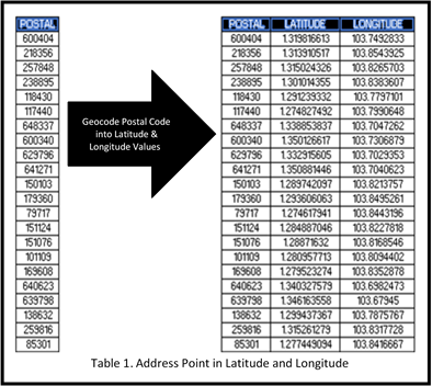
| + | In order to derive the corresponding Latitude and Longitude from the customer’s postal codes, the team utilised oneMap’s API web service. Through using spatial reference code WGS84, this API web service aided the team in generating table 1 – “Address Point”, which is a geocoded table comprising of individual postal code and their respective Latitude and Longitude values. | ||
| + | </p> | ||
| + | [[Image:TWO Table1.png | 400px | center]] | ||
| + | <p> | ||
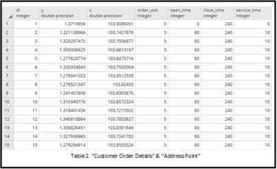
| + | By concatenating Table 1 with the Customer Order Details, the team obtained a combined table of “Customer Request Table” along with “Address Point”, which will then be loaded in PostgreSQL. | ||
| + | </p> | ||
| + | [[Image:TWO Table2.png | 400px | center]] | ||
| + | <p> | ||
| + | In addition, the team also loaded OpenStreetMap containing Singapore’s road networks into PostgreSQL. This allows the Singapore map to be populated with the road networks in Singapore as shown below. | ||
| + | </p> | ||
| + | [[Image:TWO MAP.png | 600px | center]] | ||
| + | <p> | ||
| + | The aforementioned procedures allow the “Street Network Map”, “Customer Request Table” and “Address Point” to be loaded within PostgreSQL. This ensures that the Input/Database Tier section of the framework discussed in Section 5.1 to be completed. | ||
| + | </p> | ||
| + | <br /> | ||
| + | |||
| + | <b><u>Application Tier</u></b> | ||
| + | <p> | ||
| + | In order to obtain a routing solution, the team will be using a spatial plugin from PostgreSQL – pgRouting. This plugin requires 3 tables to be formed and they are 1) Cost Metric, 2) Customer Request Table & 3) Vehicle Table. | ||
| + | </p> | ||
| + | <br /><br /> | ||
| + | 1. <b>Application Tier – Cost Metric Table</b> | ||
| + | <p> | ||
| + | The Cost Metric Table is a table indicating the distance between each pair of LocationIDs. This LocationID can be derived from geometry data which are coded from Latitude and Longitude values. | ||
| + | <br /><br /> | ||
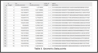
| + | Therefore, given the existing inputs, the first step is to convert geometry data from the Latitude and Longitude values obtained in Table 1. By using PostGIS, this will help convert each Latitude and Longitude values from Table 1 into a unique geometry data, as shown in Table 3. | ||
| + | </p> | ||
| + | [[Image:TWO table3.png | 400px | center]] | ||
| + | <p> | ||
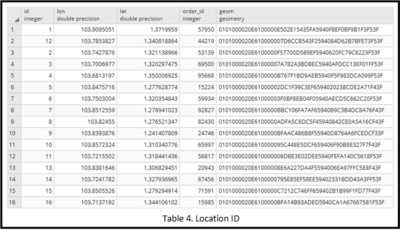
| + | When Table 3 is used in conjunction with the “Street Network Map”, obtained from OpenStreetMap, it identifies the nearest EdgeID based on the geometry data obtained earlier. This process is done with the help of PostGIS and is shown in Table 4. | ||
| + | </p> | ||
| + | [[Image:TWO table4.png | 400px | center]] | ||
| + | <p> | ||
| + | With the LocationID obtained previously, along with the renowned single-source shortest path algorithm – Dijkstra Algorithm, the Cost Metric table between each LocationID will be derived. | ||
| + | </p> | ||
| + | [[Image:TWO table5.png | 400px | center]] | ||
| + | <p> | ||
| + | However, as shown in Table 5, the units for Distance and Time are Metres and Seconds respectively. This is not in line with the requirements from pgRouting’s Vehicle Routing Problem Algorithm. Hence, it is imperative to convert the Distance units to Kilometres and Time units to Hours. | ||
| + | </p> | ||
| + | [[Image:TWO table6.png | 400px | center]] | ||
| + | <p> | ||
| + | With this, the Cost Metric Table is now ready for pgRouting’s Vehicle Routing Problem Algorithm. | ||
| + | </p> | ||
| + | |||
| + | <br/><br/> | ||
| + | |||
| + | 2. <b>Application Tier –Customer Request Table & Vehicle Table</b> | ||
| + | <p> | ||
| + | The Customer Request Table is a table indicating the Customer’s Delivery Locations (in Latitude and Longitude) along with the Opening Time, Closing Time and Service Time. This table has been generated in Table 2 and is now replicated in Table 8 below | ||
| + | <br/><br/> | ||
| + | The Vehicle Table is a table indicating the unique Vehicle IDs and its respective capacity. This table requires the manual input from the user and a sample is as shown in Table 9 below. | ||
| + | </p> | ||
| + | [[Image:TWO table7.png | 400px | center]] | ||
| + | <p> | ||
| + | After obtaining the Cost Metric, Customer Request and Vehicle Table, the user is now ready to obtain the routing solutions from pgRouting’s Vehicle Routing Problem Algorithm. | ||
| + | </p> | ||
| + | |||
| + | <br/><br/> | ||
| + | |||
| + | 3. <b>Client Interface Tier</b> | ||
| + | <p> | ||
| + | After running the Vehicle Routing Problem Algorithm, the routing output will be displayed in a table format which can be viewed on QGIS. This table, as shown in Table 10, will provide the route that each unique Vehicle ID should follow to minimise the time taken. | ||
| + | </p> | ||
| + | [[Image:TWO table8.png | 400px | center]] | ||
| + | <p> | ||
| + | However, as the table has little relevance to the user, the team have used the Dijkstra Algorithm to help identify the routes each driver should take in the form of a map. This pictorial depiction can also be viewed through QGIS and this final result represents the routing solution that the team aim to achieve. | ||
| + | </p> | ||
| + | [[Image:TWO table9.png | 500px | center]] | ||
| + | |||
</div> | </div> | ||
<!--- End Analysis Content --> | <!--- End Analysis Content --> | ||
| − | <!-- Start of | + | <!-- Start of Analysis Content --> |
{| width=1080px cellspacing="0" cellpadding="7" | {| width=1080px cellspacing="0" cellpadding="7" | ||
| − | | style="background-color:#2B6C94; font-weight: bold; text-indent: 15px; border-left: 15px solid #4BB9FF" | <font color="#FFF" size=3 > | + | | style="background-color:#2B6C94; font-weight: bold; text-indent: 15px; border-left: 15px solid #4BB9FF" | <font color="#FFF" size=3 > User Interface</font> |
|} | |} | ||
<br /> | <br /> | ||
| − | <div style=" | + | <div style="padding-left:70px; text-align: justify; width:980px;"> |
| − | < | + | <p> |
| + | Given that the following methodology can derive a routing solution for Company ABC, this section will now focus on providing a user-friendly interface through R’s interactive web app package – Shiny. This interface allows user to derive routing solutions in 9 steps. | ||
| + | </p> | ||
| + | |||
| + | |||
| + | <p> | ||
| + | <b><u>Step 1: </u></b> Select “Choose File” Button on the User Interface to upload the Customer Order Data. | ||
| + | </p> | ||
| + | [[Image:TWO step1.png | 500px | center]] | ||
| + | <p> | ||
| + | <b><u>Step 2: </u></b> Select Order Details file from the Local Work Station. Ensure that this file is in “.csv” format. | ||
| + | </p> | ||
| + | [[Image:TWO step2.png | 500px | center]] | ||
| + | <p> | ||
| + | <b><u>Step 3: </u></b> Upon choosing the relevant file, click on the “Upload and Geocode” button. | ||
| + | </p> | ||
| + | [[Image:TWO step3.png | 500px | center]] | ||
| + | <p> | ||
| + | <b><u>Step 4: </u></b> After selecting the “Upload and Geocode” button, this would help create the data table containing Latitude, Longitude, Opening Time, Closing Time and Service Time. | ||
| + | </p> | ||
| + | [[Image:TWO step4.png | 500px | center]] | ||
| + | <p> | ||
| + | <b><u>Step 5: </u></b> Next click on the Vehicle Table tab to begin inputs for Vehicle Table. | ||
| + | </p> | ||
| + | [[Image:TWO step5.png | 500px | center]] | ||
| + | <p> | ||
| + | <b><u>Step 6: </u></b> Choose the Vehicle Table file from the Local Work Station. | ||
| + | </p> | ||
| + | [[Image:TWO step6.png | 500px | center]] | ||
| + | <p> | ||
| + | <b><u>Step 7: </u></b> Upon selecting the file, click “Upload” to display the Vehicle Table File in the interface | ||
| + | </p> | ||
| + | [[Image:TWO step7.png | 500px | center]] | ||
| + | <p> | ||
| + | <b><u>Step 8: </u></b> Select on “VRP Routing” tab to generate the routing solution in a table format. The Routing Table would provide the delivery details such as the time each driver should arrive and depart at each location. This will also create a new tab know as “Routes” which provides the solution in a map. | ||
| + | </p> | ||
| + | [[Image:TWO step8.png | 500px | center]] | ||
| + | <p> | ||
| + | <b><u>Step 9: </u></b> By selecting the new tab called “Routes”, this will provide the output as shown in the diagram below (Figure 14). The Routing map, unlike the Routing Table, would be a pictorial depiction of the routes that each driver should be taking. This tab, thus, provides the management with a strategic perspective on the routes that each driver would take. | ||
| + | </p> | ||
| + | [[Image:TWO step9.png | 500px | center]] | ||
| + | <p> | ||
| + | <b><u>Step 10: </u></b> In order to be more interactive, the team explored using QGIS to utilise the filters provided. This allows the company to identify the routes that each individual driver should take, which would be valuable for the company. | ||
| + | </p> | ||
| + | [[Image:TWO step10.png | 500px | center]] | ||
</div> | </div> | ||
| − | <!--- End | + | <!--- End Analysis Content --> |
| + | |||
</center> | </center> | ||
<br /> | <br /> | ||
<br /> | <br /> | ||
Latest revision as of 00:19, 16 April 2018
| HOME | PROJECT OVERVIEW | ANALYSIS & INSIGHTS | PROJECT MANAGEMENT | DOCUMENTATION | ANLY482 MAIN |
| EDA | ANALYSIS & INSIGHTS |
|---|
| Model Building |
Inputs/Database Tier
In order to derive the corresponding Latitude and Longitude from the customer’s postal codes, the team utilised oneMap’s API web service. Through using spatial reference code WGS84, this API web service aided the team in generating table 1 – “Address Point”, which is a geocoded table comprising of individual postal code and their respective Latitude and Longitude values.
By concatenating Table 1 with the Customer Order Details, the team obtained a combined table of “Customer Request Table” along with “Address Point”, which will then be loaded in PostgreSQL.
In addition, the team also loaded OpenStreetMap containing Singapore’s road networks into PostgreSQL. This allows the Singapore map to be populated with the road networks in Singapore as shown below.
The aforementioned procedures allow the “Street Network Map”, “Customer Request Table” and “Address Point” to be loaded within PostgreSQL. This ensures that the Input/Database Tier section of the framework discussed in Section 5.1 to be completed.
Application Tier
In order to obtain a routing solution, the team will be using a spatial plugin from PostgreSQL – pgRouting. This plugin requires 3 tables to be formed and they are 1) Cost Metric, 2) Customer Request Table & 3) Vehicle Table.
1. Application Tier – Cost Metric Table
The Cost Metric Table is a table indicating the distance between each pair of LocationIDs. This LocationID can be derived from geometry data which are coded from Latitude and Longitude values.
Therefore, given the existing inputs, the first step is to convert geometry data from the Latitude and Longitude values obtained in Table 1. By using PostGIS, this will help convert each Latitude and Longitude values from Table 1 into a unique geometry data, as shown in Table 3.
When Table 3 is used in conjunction with the “Street Network Map”, obtained from OpenStreetMap, it identifies the nearest EdgeID based on the geometry data obtained earlier. This process is done with the help of PostGIS and is shown in Table 4.
With the LocationID obtained previously, along with the renowned single-source shortest path algorithm – Dijkstra Algorithm, the Cost Metric table between each LocationID will be derived.
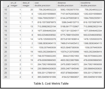
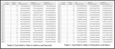
However, as shown in Table 5, the units for Distance and Time are Metres and Seconds respectively. This is not in line with the requirements from pgRouting’s Vehicle Routing Problem Algorithm. Hence, it is imperative to convert the Distance units to Kilometres and Time units to Hours.
With this, the Cost Metric Table is now ready for pgRouting’s Vehicle Routing Problem Algorithm.
2. Application Tier –Customer Request Table & Vehicle Table
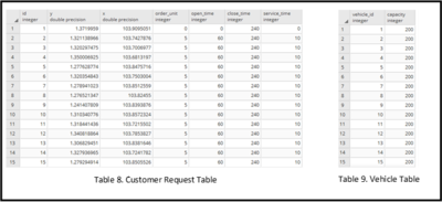
The Customer Request Table is a table indicating the Customer’s Delivery Locations (in Latitude and Longitude) along with the Opening Time, Closing Time and Service Time. This table has been generated in Table 2 and is now replicated in Table 8 below
The Vehicle Table is a table indicating the unique Vehicle IDs and its respective capacity. This table requires the manual input from the user and a sample is as shown in Table 9 below.
After obtaining the Cost Metric, Customer Request and Vehicle Table, the user is now ready to obtain the routing solutions from pgRouting’s Vehicle Routing Problem Algorithm.
3. Client Interface Tier
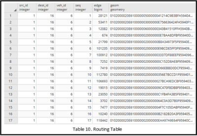
After running the Vehicle Routing Problem Algorithm, the routing output will be displayed in a table format which can be viewed on QGIS. This table, as shown in Table 10, will provide the route that each unique Vehicle ID should follow to minimise the time taken.
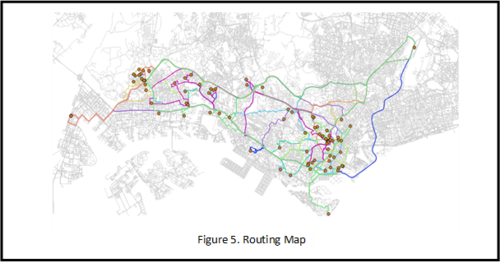
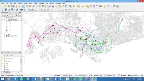
However, as the table has little relevance to the user, the team have used the Dijkstra Algorithm to help identify the routes each driver should take in the form of a map. This pictorial depiction can also be viewed through QGIS and this final result represents the routing solution that the team aim to achieve.
| User Interface |
Given that the following methodology can derive a routing solution for Company ABC, this section will now focus on providing a user-friendly interface through R’s interactive web app package – Shiny. This interface allows user to derive routing solutions in 9 steps.
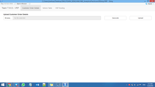
Step 1: Select “Choose File” Button on the User Interface to upload the Customer Order Data.
Step 2: Select Order Details file from the Local Work Station. Ensure that this file is in “.csv” format.
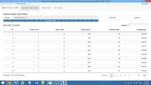
Step 3: Upon choosing the relevant file, click on the “Upload and Geocode” button.
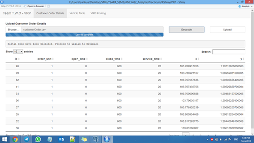
Step 4: After selecting the “Upload and Geocode” button, this would help create the data table containing Latitude, Longitude, Opening Time, Closing Time and Service Time.
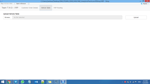
Step 5: Next click on the Vehicle Table tab to begin inputs for Vehicle Table.
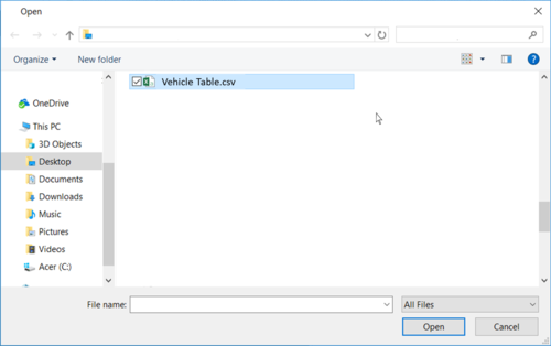
Step 6: Choose the Vehicle Table file from the Local Work Station.
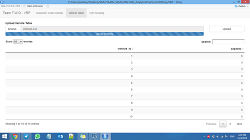
Step 7: Upon selecting the file, click “Upload” to display the Vehicle Table File in the interface
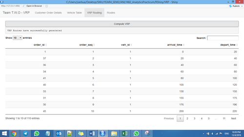
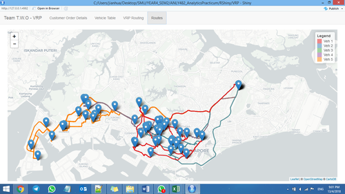
Step 8: Select on “VRP Routing” tab to generate the routing solution in a table format. The Routing Table would provide the delivery details such as the time each driver should arrive and depart at each location. This will also create a new tab know as “Routes” which provides the solution in a map.
Step 9: By selecting the new tab called “Routes”, this will provide the output as shown in the diagram below (Figure 14). The Routing map, unlike the Routing Table, would be a pictorial depiction of the routes that each driver should be taking. This tab, thus, provides the management with a strategic perspective on the routes that each driver would take.
Step 10: In order to be more interactive, the team explored using QGIS to utilise the filters provided. This allows the company to identify the routes that each individual driver should take, which would be valuable for the company.

