Difference between revisions of "ANLY482 AY2016-17 T2 Group20 Findings"
| Line 49: | Line 49: | ||
==== Unclean variable – modelName ==== | ==== Unclean variable – modelName ==== | ||
| + | [[File:ModelName_Dist.png|frameless|300px]] | ||
| + | [[File:CleanModelName_Dist.png|frameless|300px]] | ||
When we looked at the summary statistics of modelName, we can see that there are a few categories which should belong in another. For example, in the screenshot above, you can see that there are many 3 Series trims such as ‘318’, ‘323’, ‘325i’ which should belong in the ‘3 Series’ category so should be relabeled to ‘3 Series’. | When we looked at the summary statistics of modelName, we can see that there are a few categories which should belong in another. For example, in the screenshot above, you can see that there are many 3 Series trims such as ‘318’, ‘323’, ‘325i’ which should belong in the ‘3 Series’ category so should be relabeled to ‘3 Series’. | ||
| Line 107: | Line 109: | ||
|- | |- | ||
|} | |} | ||
| + | |||
| + | We chose to remove the rows which have missing values of ‘currentPriceOther’ since that is the target variable. Without data from the target variable, the row would be unable to be used in the model. After removing the rows with missing values of ‘currentPriceOther’, we can see that there is a significantly lower percentage of missing values. | ||
| + | |||
| + | ==== Removing Outliers ==== | ||
| + | Outliers have extreme values that can largely influence our statistical analysis. While it may represent natural variation in our data, we decided to set the standard in classifying a data point as an outlier by using the Quantile Range Outliers in JMP. We chose Quantile Range Outliers instead of the other 3 possible choices such as Robust Fit Options, Multivariate Robust outliers and Multivariate k-Nearest Neighbor Outliers because the Quantile Range Outliers does not assume distribution associated with the data. Extreme values are calculated using the multiplier of the interquartile range(IQR). | ||
| + | |||
| + | We used a value of 0.1 for the Tail Quantile, and 4 for Q, which means in identifying the outliers, values have to be 4 times for than the IQR. All the values in the low threshold is negative,which means only the high threshold is considered as a qualifier. | ||
| + | |||
| + | {| class="wikitable" | ||
| + | |- | ||
| + | ! Variable !! High Threshold !! Max Value !! No. of outliers !! Explanation | ||
| + | |- | ||
| + | | daysCount || 408 || 522 || 117 || In building a pricing model, we are looking at used cars that have a reasonable days to market period. For these cars beyond more than a year, cases of such car existing could be due to: | ||
| + | # Vintage cars | ||
| + | # Small dealerships - “Some small dealerships could be storing it in a warehouse or empty space, these cars are not maintained” - Steve Greenfield, CEO of Automotive Ventures | ||
| + | |||
| + | Hence it may not be a relevant indicator for our pricing model. | ||
| + | |- | ||
| + | | currentMsrp || 193,572 || 1,056,454 || 3 || Blanket rule for a generalised model. | ||
| + | |- | ||
| + | | currentPriceOther || 196,506 || 955,719 || 4 || Blanket rule for a generalised model. | ||
| + | |- | ||
| + | | mileage || 287,275 || 962,525 || 23 || Cars driven beyond 200,000 miles are considered the high mileage for used cars. https://www.reference.com/vehicles/considered-high-mileage-car-e661f36f0817e76b | ||
| + | |} | ||
| + | |||
| + | We did not consider removing outliers for msrpCount, priceOtherCount and Age because these are calculated variables based on the initial variables in currentMsrp, currentPriceOther and for year variable, we are not removing the possibilities of vintage cars which can be manufactured in 1983. | ||
| + | |||
| + | Another advantage of Quantile Range Outliers is that it identifies the Nines. In most industries, a high value of 999999 is commonly used to fill in for a missing value. Though our analysis we found that the number of nines found in the dataset does not reflect that it has been used to recode for missing variables. The highest count was 3603, and it was found for Age, which reflects cars that have been produced in 2008. In addition, we consulted with the developers to how they have recoded missing values, where it is left as it is. | ||
| + | |||
| + | |||
| + | |||
| + | In conclusion, the total no. of outliers removed are insignificant compared to our dataset, hence we chose to remove the abovementioned outliers. | ||
Revision as of 23:47, 19 February 2017
Working documents
- Example of analysis: File:RegressionBMW.xlsx
- Example of R code: File:RegressionBMW.txt
Contents
Data Exploration and Cleaning
Issues
Too large dataset
Due to the large dataset, it took too long to run the nodes in SAS Enterprise Miner which resulted in the inefficiency. It took approximately 6 hours to run a single node.
We reduced the dataset to BMW cars by filtering the dataset “makeName = BMW” and “used=1,2” to retrieve a dataset result of used BMW cars. We categorized the BMW cars based on the ‘modelName’, where the cleaning and categorization of ‘modelName’ will be explained below. Throughout the project, we will be using BMW cars as a model while keeping it generalised. Thereafter, we will be using the same model as a template for other car brands. This can be done by filtering the ‘makeName’ column which uses brand as the main filter.
This reduces the load on the system as we will only be using BMW cars for analysis.
Customers would already have a preferred car brand based on their buying capacity and personal preference for cars. From the general model, dealers will be able to select the car brands (“makeName”) of the customers’ preference, which will lead them to the specifications (“modelName”) of the car.
Unclean variable – modelName
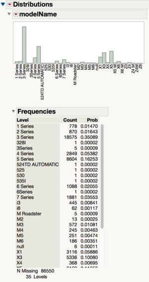
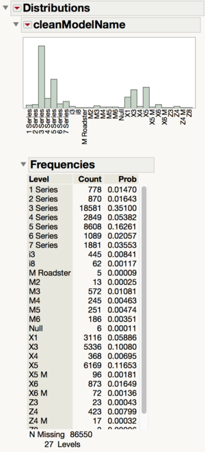
When we looked at the summary statistics of modelName, we can see that there are a few categories which should belong in another. For example, in the screenshot above, you can see that there are many 3 Series trims such as ‘318’, ‘323’, ‘325i’ which should belong in the ‘3 Series’ category so should be relabeled to ‘3 Series’.
Missing Values
| Column | Number Missing (before) | Percentage Missing (before) | Number Missing (after) | Percentage Missing (after) |
|---|---|---|---|---|
| year | 0 | 0.00% | 0 | 0.00% |
| minDate | 0 | 0.00% | 0 | 0.00% |
| maxDate | 0 | 0.00% | 0 | 0.00% |
| daysCount | 0 | 0.00% | 0 | 0.00% |
| currentMsrp | 74357 | 53.31% | 14127 | 26.69% |
| currentPriceOther | 86550 | 62.05% | 0 | 0.00% |
| minMsrp | 65831 | 47.20% | 9232 | 17.44% |
| maxMsrp | 66243 | 47.49% | 9312 | 17.59% |
| msrpCount | 0 | 0.00% | 0 | 0.00% |
| minPriceOther | 78926 | 56.58% | 154 | 0.29% |
| maxPriceOther | 78937 | 56.59% | 164 | 0.31% |
| priceOtherCount | 0 | 0.00% | 0 | 0.00% |
| sold | 0 | 0.00% | 0 | 0.00% |
| used | 0 | 0.00% | 0 | 0.00% |
| mileage | 49438 | 35.44% | 1924 | 3.63% |
| Sq Root[mileage] | 49438 | 35.44% | 1924 | 3.63% |
| Log[mileage] | 54259 | 38.90% | 4482 | 8.47% |
| Log10[mileage] | 54259 | 38.90% | 4482 | 8.47% |
| Cube Root[mileage] | 49438 | 35.44% | 1924 | 3.63% |
| vehicleAge | 0 | 0.00% | 0 | 0.00% |
| Square Root[vehicleAge] | 9 | 0.01% | 3 | 0.01% |
| Log10[vehicleAge] | 4301 | 3.08% | 2705 | 5.11% |
| Log[vehicleAge] | 4301 | 3.08% | 2705 | 5.11% |
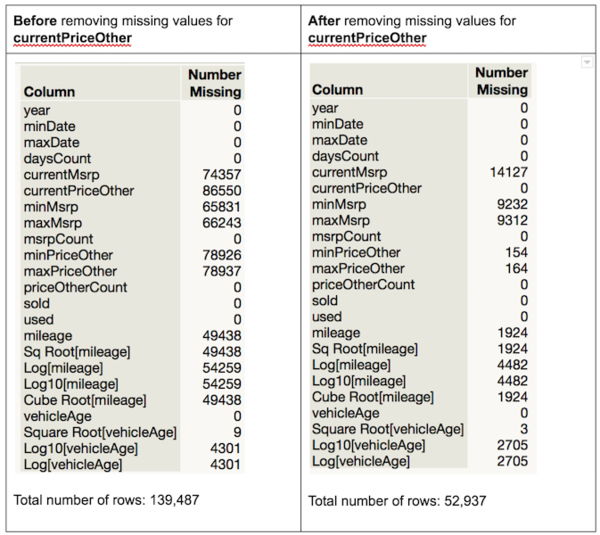
We chose to remove the rows which have missing values of ‘currentPriceOther’ since that is the target variable. Without data from the target variable, the row would be unable to be used in the model. After removing the rows with missing values of ‘currentPriceOther’, we can see that there is a significantly lower percentage of missing values.
Removing Outliers
Outliers have extreme values that can largely influence our statistical analysis. While it may represent natural variation in our data, we decided to set the standard in classifying a data point as an outlier by using the Quantile Range Outliers in JMP. We chose Quantile Range Outliers instead of the other 3 possible choices such as Robust Fit Options, Multivariate Robust outliers and Multivariate k-Nearest Neighbor Outliers because the Quantile Range Outliers does not assume distribution associated with the data. Extreme values are calculated using the multiplier of the interquartile range(IQR).
We used a value of 0.1 for the Tail Quantile, and 4 for Q, which means in identifying the outliers, values have to be 4 times for than the IQR. All the values in the low threshold is negative,which means only the high threshold is considered as a qualifier.
| Variable | High Threshold | Max Value | No. of outliers | Explanation |
|---|---|---|---|---|
| daysCount | 408 | 522 | 117 | In building a pricing model, we are looking at used cars that have a reasonable days to market period. For these cars beyond more than a year, cases of such car existing could be due to:
Hence it may not be a relevant indicator for our pricing model. |
| currentMsrp | 193,572 | 1,056,454 | 3 | Blanket rule for a generalised model. |
| currentPriceOther | 196,506 | 955,719 | 4 | Blanket rule for a generalised model. |
| mileage | 287,275 | 962,525 | 23 | Cars driven beyond 200,000 miles are considered the high mileage for used cars. https://www.reference.com/vehicles/considered-high-mileage-car-e661f36f0817e76b |
We did not consider removing outliers for msrpCount, priceOtherCount and Age because these are calculated variables based on the initial variables in currentMsrp, currentPriceOther and for year variable, we are not removing the possibilities of vintage cars which can be manufactured in 1983.
Another advantage of Quantile Range Outliers is that it identifies the Nines. In most industries, a high value of 999999 is commonly used to fill in for a missing value. Though our analysis we found that the number of nines found in the dataset does not reflect that it has been used to recode for missing variables. The highest count was 3603, and it was found for Age, which reflects cars that have been produced in 2008. In addition, we consulted with the developers to how they have recoded missing values, where it is left as it is.
In conclusion, the total no. of outliers removed are insignificant compared to our dataset, hence we chose to remove the abovementioned outliers.


