Qui Vivra Verra - Project Findings
Further analysis of the data set can be accomplished through market segmentation. The concept of k-means clustering can be applied on the Transaction Dataset, with the clustering parameters set as:
- Recency (number of days from last transaction to end of the FY)
- Frequency (number of transactions performed within the FY)
- Monetary (average number of books borrowed per transaction)
Each patron will then be assigned to a cluster, with each cluster homogeneous within and heterogeneous across. From here, we can determine the dominant cluster of library member that each library caters to – which can provide some operational insights by understanding the demographics of the bulk of each library’s patrons.
The Huff’s Model is a gravity model that is capable of estimating the probability of a consumer patronising a shopping area, out of a list of shopping areas. First developed by David Huff (1964), it has its base on several important consumer-flow patterns that are generally true:
- The proportion of consumers patronizing a given shopping area varies with distance from the shopping area
- The proportion of consumers patronizing various shopping areas varies with the breadth and depth of merchandise offered by each shopping area
- The distance that consumers travel to various shopping areas vary for different types of product purchases
- The “pull” of any given shopping area is influenced by the proximity of competing shopping areas
On top of these empirical trends, the Huff’s Model attempts to mathematically derive an equation which seeks to explain the consumer spatial pattern, while taking into considering all possible shopping areas (Huff, 1964).
Since then, there have been many adaptations and improvements of the model to suit the peculiarity of each case it was applied on. Suárez-Vega, Gutiérrez-Acuña, & Rodríguez-Díaz. (2015) mentioned that the global parameters (attractiveness index and distance decay) calibrated by the Huff’s Model are global, and is assumed to hold over the entire area of interest. However, there may be variations at different regions which may give rise to local differences in the attractiveness of the retail areas. Then, they presented an adaption which shows spatial non-stationarity, which is capable of giving local information about the consumers which the global model ignores.
In their summary paper, Roy & Thill (2003) mentioned the replacement of the distance variable with the transport cost variable, represented by both time and monetary terms, while taking into account the level of accessibility in different areas. Instead of the Ordinary Least Squares (OLS) method which a due transformation of the general equation of the Huff’s Model is able to work with, other optimization methods such as entropy and artificial neural networks were considered (Roy & Thrill, 2003). The concept of opportunity cost in terms of transport cost to a nearby retail destination is also mentioned in their paper (Roy & Thrill, 2003).
To increase the predictive accuracy of the model, Okabe & Sugihara (2012) used the shortest-path distance of a street network instead of the Euclidean distance in the original Huff’s Model. As the relevant transportation time and monetary costs will fit actuality to a greater extent, this variant may be preferred in areas where the commuting pattern of consumers has a high correlation with the street network. Furthermore, to estimate the actual density of consumer flow, Okabe & Sugihara (2012) integrated the choice probability derived from their variant of the Huff’s Model over the density of consumers in the whole market area. This will generate insights on the absolute amount of consumer flow to a given retail trade area, effectively a useful extension of the original Huff’s Model. An adaptation of the Huff’s Model (Huff, 1964) will be applied in the analyses.
To quote a paper by Okabe & Sugihara (2012):
To state a general form of the Huff model, we consider a space S (which may be a plane or a network), in which n stores are located at p1, …, pn. Let ai be the attractiveness of store i, which may be a function of its floor area, the number of items sold, its parking area and so forth; let d(p, pi) be the distance between a point p on S and the store at pi, which may be the Euclidean distance or the shortest-path distance; and let F(d(p, pi)) be a monotonically decreasing function of d(p, pi), referred to as a distance decay function or distance deterrence function. In these terms, the Huff model showing the probability of a consumer at p choosing the store at pi is generally written as:
Adapting the Huff’s Model to the context of our project, we would consider Singapore as space S, in which n libraries are located at p1, …, pn. Let ai be the attractiveness of library i, which is estimated by a multinomial generalised linear regression equation, taking into account the following factors (non-exhaustive):
- Size of the library’s collection
- Gross floor area of the library
- Type of facility the library is located in (i.e. mall, stand-alone etc)
- Size of facility the library is in (i.e. if the library is located in a mall, this refers to the gross floor area of the mall)
- Number of MRT stations within a set distance (to be determined) from the library
- Number of bus stops within a set distance (to be determined) from the library
- Number of bus routes within a set distance (to be determined) from the library
- Opening hours of the library
- Number of educational institutes (i.e. primary/secondary schools, junior colleges, polytechnics, ITE, universities) within a set distance (to be determined) from the library
- Number of other libraries (only considering the list under NLB) within a set distance from the library
Let d(p, pi) be the distance between an area (geographical subzone) p on S and the library at pi, which may be the Euclidean distance or the shortest-path distance; and let F(d(p, pi)) be a monotonically decreasing function of d(p, pi), referred to as a distance decay function or distance deterrence function. Therefore, the above-stated formula can be interpreted as the probability of a consumer at p choosing the library at pi.
Dividing the number of patrons in each subzone at p that visited a library pi by the total number of patrons in the subzone at p, we can obtain a probabilistic model which estimates the proportion of time that a patron from subzone p will visit library i in any given FY. Then, by substituting the known values of ai (to be determined by the regression model) and d(p, pi) into the adapted Huff’s Model, we are able to derive possible values of the power parameter (∝) that govern the distance decay function. By doing this process iteratively, we can obtain an unbiased estimate for ∝ that is accurate to a certain significant level.
Measures of Demand
We are able to measure the demand of a given library relative to all other libraries, using 2 different proxies:
- Proportion of books borrowed from library by subzone
- Proportion of transactions from library by subzone
Proportion of Books Borrowed from Library by Subzone
Using the 2013 Transactions Dataset, we identified 270 unique subzone categories. For each subzone category (e.g. AMSZ01, AMSZ02, etc.), we derived the no. of books borrowed from each library in FY2013. Thereafter, we calculated the total no. of books borrowed (from all the libraries) by each subzone. Hence, we are able to calculate the proportion of books borrowed from each library by a given subzone by using the formula:
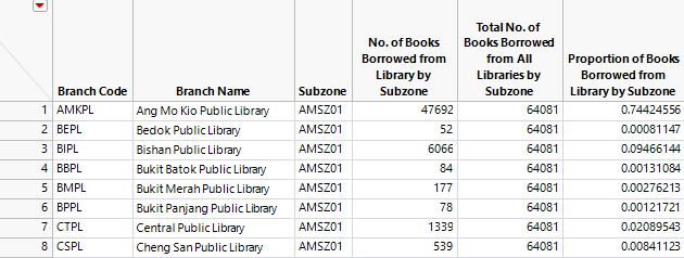
A snapshot of the calculated field is as shown below.
For example, patrons residing in AMSZ01 have borrowed a total of 47,692 books from AMKPL. Patrons residing in AMSZ01 have borrowed a total of 64,081 books from all the libraries in FY2013. Hence, approximately 74.4% of all books borrowed by patrons residing in AMSZ01 are borrowed from AMKPL.
Proportion of Transactions from Library by Subzone
In a similar sense, for each subzone category (e.g. AMSZ01, AMSZ02, etc.), we derived the no. of transactions from each library in FY2013. Thereafter, we calculated the total no. of transactions (from all the libraries) by each subzone. Hence, we are able to calculate the proportion of transactions from each library by a given subzone by using the formula:
A snapshot of the calculated field is as shown below.
For example, patrons residing in AMSZ01 performed a total of 8,710 transactions from AMKPL. Patrons residing in AMSZ01 performed a total of 12,347 transactions from all the libraries in FY2013. Hence, approximately 70.5% of all transactions performed by patrons residing in AMSZ01 are performed at AMKPL.
Distance from Library to Planning Area Centroid
Using the data on latitudes and longitudes of each library and each planning area centroid, we used the spherical law of cosines formula to calculate the distance from a given planning area centroid to each library. A snapshot of the data is shown below.
For example, AMKPL is approximately 0.705km from the Ang Mo Kio Planning Area Centroid.
Next, we performed a regression analysis to discover the relationship (if any) of the attractive index of a library (described by the characteristics of a library and its nearby amenities) and the distance from a library to a given planning area centroid on the demand of the library for a given subzone.
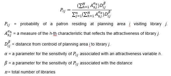
Let the general form of the Huff’s Model be:
We seek to find the optimal values of α and β. In order to have statistical verification in our analysis, we will be employing the Ordinary Least Squared (OLS) regression. To do so, first we need to linearize the equation by performing some transformations:
We start by taking the logarithm of the general form:
Summing both sides over j (= 1, 2, …, n), and dividing both sides by n, we have:
Demand as the Proportion of Books Borrowed from Library
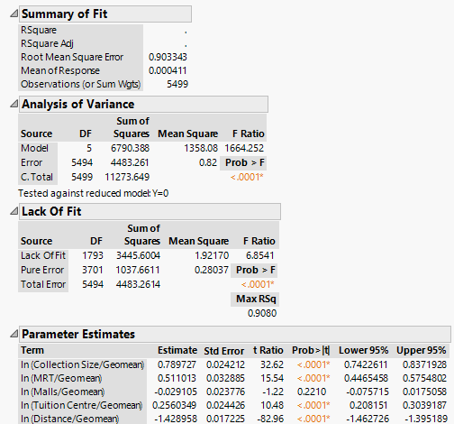
Using the 2013 Transaction Dataset, we ran an OLS regression, excluding the intercept term. A summary of the results is shown in the diagram below.
We first note that the alpha values for Collection Size, No. of MRT within 1km, No. of Tuition Centres within 1km are positive. This aligns with our expectations, as these variables correlate positively with the attractiveness index of a given library. All of the coefficients are statistically significant at the 1% significance level (p < 0.01). However, the alpha value for No. of Shopping Malls within 1km is not statistically significant at the 1% significance level. Next, we note that the beta value (i.e. distance decay parameter) is estimated to be -1.428958, which also aligns with our expectations; we expect a greater distance from a given library would reduce the probability that a patron will patronise the library.
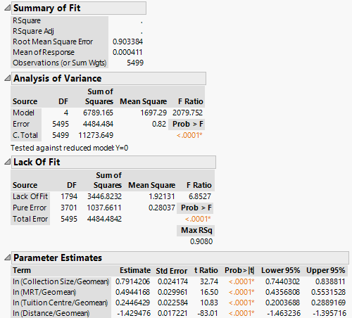
Next, we drop the ln (Tuition Centre/Geomean) term and re-ran the regression with results as shown below:
The coefficient estimates of the remaining variables differed by a slight amount, while the signs and statistical significances remain as before.
Therefore, we can estimate the probability of a patron residing at planning area i visiting library j using the equation, with the estimated parameters:
Demand as the Proportion of Transactions from Library
As there are different proxies to estimate the demand for a given library, we explored the possibility of an alternative regression model which uses the proportion of transactions from a library by a given subzone.
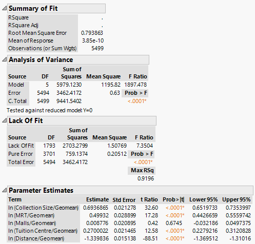
Using the 2013 Transaction Dataset, we ran an OLS regression, excluding the intercept term. A summary of the results is shown in the diagram below.
We first note that the alpha values for Collection Size, No. of MRT within 1km, No. of Tuition Centres within 1km are positive. This aligns with our expectations, as these variables correlate positively with the attractiveness index of a given library. All of the coefficients are statistically significant at the 1% significance level (p < 0.01). However, the alpha value for No. of Shopping Malls within 1km is not statistically significant at the 1% significance level.
Next, we note that the beta value (i.e. distance decay parameter) is estimated to be -1.339836, which also aligns with our expectations; we expect a greater distance from a given library would reduce the probability that a patron will patronise the library.
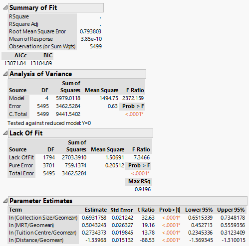
Next, we drop the ln (Tuition Centre/Geomean) term and re-ran the regression with results as shown below:
The coefficient estimates of the remaining variables differed by a slight amount, while the signs and statistical significances remain as before.
Therefore, we can estimate the probability of a patron residing at planning area i visiting library j using the equation, with the estimated parameters:
Demand as the Proportion of Books Borrowed from Library Residual Analysis
We first visualize the relationship between the actual response variable and predicted response variable. We observe a root-mean-square error (RMSE) of 0.9034.
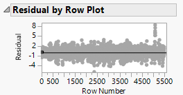
Next, we plotted the residual by predicted and residual by row, to check for non-constant variation across the data. We observe that there is no constant variation of the residual across different predicted values, and different rows. There is also no obvious evidence of heteroscedasticity in the regression.
Cross-validation on 2014 Data
With the appropriate estimates of the parameters, we predict the probability of a patron residing in planning area i visiting library j by using the equation:
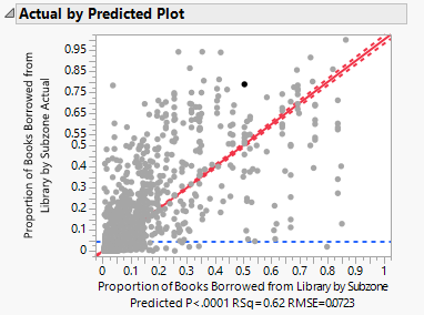
Plotting the actual proportion of books borrowed from library by subzone on the predicted values, we get the following results:
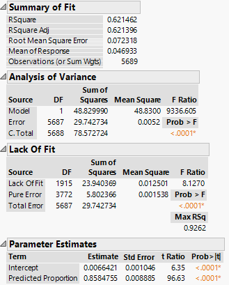
An R-Square value of 0.621462 tells us that approximately 62.15% of the variations in the actual values are explained by the predicted values. The remaining 37.84% are unexplained by the model.
For both the ANOVA and Lack-of-Fit analyses, the F-statistics are statistically significant at the 0.1% significance level, which suggests that the model is functional.
For the parameter estimates, we expected the estimate for the predicted proportion to be 1. The results show that it is 0.8584755, which is lower than 1, suggesting that on average there is over-estimation of the predicted proportion.
Next we perform a distribution analysis on the residual (i.e. actual minus predicted). The results align with our expectations, that the residual approximately follows a normal distribution with mean nearing 0. This suggests that there is no heteroscedasticity present in the regression model.
Demand as the Proportion of Transactions from Library Residual Analysis
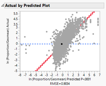
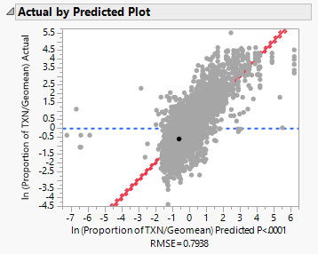
We first visualize the relationship between the actual response variable and predicted response variable. We observe a root-mean-square error (RMSE) of 0.7938. This value is lower than that of the previous model.
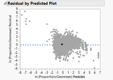
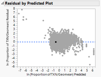
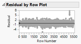
Next, we plotted the residual by predicted and residual by row, to check for non-constant variation across the data. We observe that there is no constant variation of the residual across different predicted values, and different rows. There is also no obvious evidence of heteroscedasticity in the regression.
Cross-validation on 2014 Data
With the appropriate estimates of the parameters, we predict the probability of a patron residing in planning area i visiting library j by using the equation:
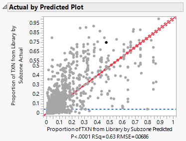
Plotting the actual proportion of books borrowed from library by subzone on the predicted values, we get the following results:
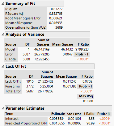
An R-Square value of 0.63277 tells us that approximately 63.28% of the variations in the actual values are explained by the predicted values. The remaining 36.72% are unexplained by the model.
For both the ANOVA and Lack-of-Fit analyses, the F-statistics are statistically significant at the 0.1% significance level, which suggests that the model is functional.
For the parameter estimates, we expected the estimate for the predicted proportion to be 1. The results show that it is 0.8815656, which is lower than 1, suggesting that on average there is over-estimation of the predicted proportion.
Next we perform a distribution analysis on the residual (i.e. actual minus predicted). The results align with our expectations, that the residual approximately follows a normal distribution with mean nearing 0. This suggests that there is no heteroscedasticity present in the regression model.
Room for Improvement
Comparing both models, using the proportion of transactions as a proxy for library demand yields a lower RMSE of 0.7938 compared to 0.9034 of the first model we looked at. Furthermore, the estimate of the predicted proportion is nearer to 1 than the first model too. However, both models have similar properties to allow us to estimate the demand for a given library. As both regressions are valid and have good prediction ability, we will employ the model that uses the proportion of books borrowed as a proxy for library demand.
In conclusion, the Huff’s Model calibrated presents a good estimation on the probability that a patron residing in planning area i visiting library j. To refine the model further, there are a few other things we can do:
- Use distance from patron’s subzone centroid to library
- Use distance from patron’s actual residence to library
- Include more variables that account for the attractiveness of a library
The above-mentioned tasks are more data-intensive than the one conducted, and we will evaluate the plausibility of including them in the dashboard visualization.
Using Distance from Library to Subzone Centroid
In an attempt to increase the predictive power of the model, we replaced the initial distance measure (from planning area centroid to library) to one which is more precise (from subzone centroid to library).
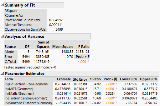
Using the 2013 Transaction Dataset, we ran an OLS regression, excluding the intercept term. A summary of the results is shown in the diagram below.
We first note that the alpha values for Collection Size, No. of MRT within 1km, No. of Tuition Centres within 1km are positive. This aligns with our expectations, as these variables correlate positively with the attractiveness index of a given library. All of the coefficients are statistically significant at the 1% significance level (p < 0.01). However, the alpha value for No. of Shopping Malls within 1km is not statistically significant at the 1% significance level.
Next, we note that the beta value (i.e. distance decay parameter) is estimated to be -1.594435, which also aligns with our expectations; we expect a greater distance from a given library would reduce the probability that a patron will patronise the library.
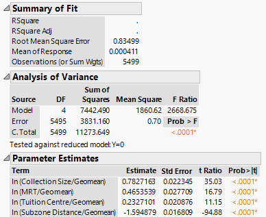
Next, we drop the ln (Tuition Centre/Geomean) term and re-ran the regression with results as shown below:
The coefficient estimates of the remaining variables differed by a slight amount, while the signs and statistical significances remain as before.
Therefore, we can estimate the probability of a patron residing at planning area i visiting library j using the equation, with the estimated parameters:
Residual Analysis
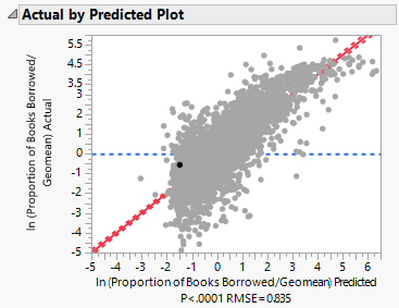
We first visualize the relationship between the actual response variable and predicted response variable. We observe a root-mean-square error (RMSE) of 0.835.
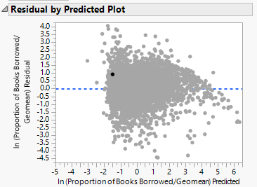
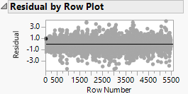
Next, we plotted the residual by predicted and residual by row, to check for non-constant variation across the data. We observe that there is no constant variation of the residual across different predicted values, and different rows. There is also no obvious evidence of heteroscedasticity in the regression.
Cross-validation on 2014 Data
With the appropriate estimates of the parameters, we predict the probability of a patron residing in planning area i visiting library j by using the equation:
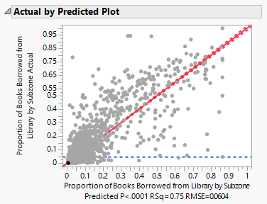
Plotting the actual proportion of books borrowed from library by subzone on the predicted values, we get the following results:
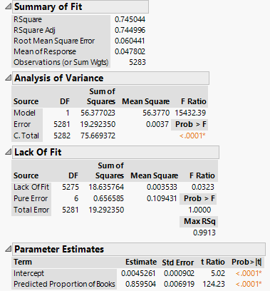
An R-Square value of 0.745044 tells us that approximately 74.5% of the variations in the actual values are explained by the predicted values. The remaining 25.5% are unexplained by the model.
For both the ANOVA and Lack-of-Fit analyses, the F-statistics are statistically significant at the 0.1% significance level, which suggests that the model is functional.
For the parameter estimates, we expected the estimate for the predicted proportion to be 1. The results show that it is 0.859504, which is lower than 1, suggesting that on average there is over-estimation of the predicted proportion.
Next we perform a distribution analysis on the residual (i.e. actual minus predicted). The results align with our expectations, that the residual approximately follows a normal distribution with mean nearing 0. This suggests that there is no heteroscedasticity present in the regression model.
All the content mentioned above will be implemented in the geospatial dashboard.

