Knowledge Discovery in Global Container Shipping Databases Findings & Insights
Contents
Overview Analysis
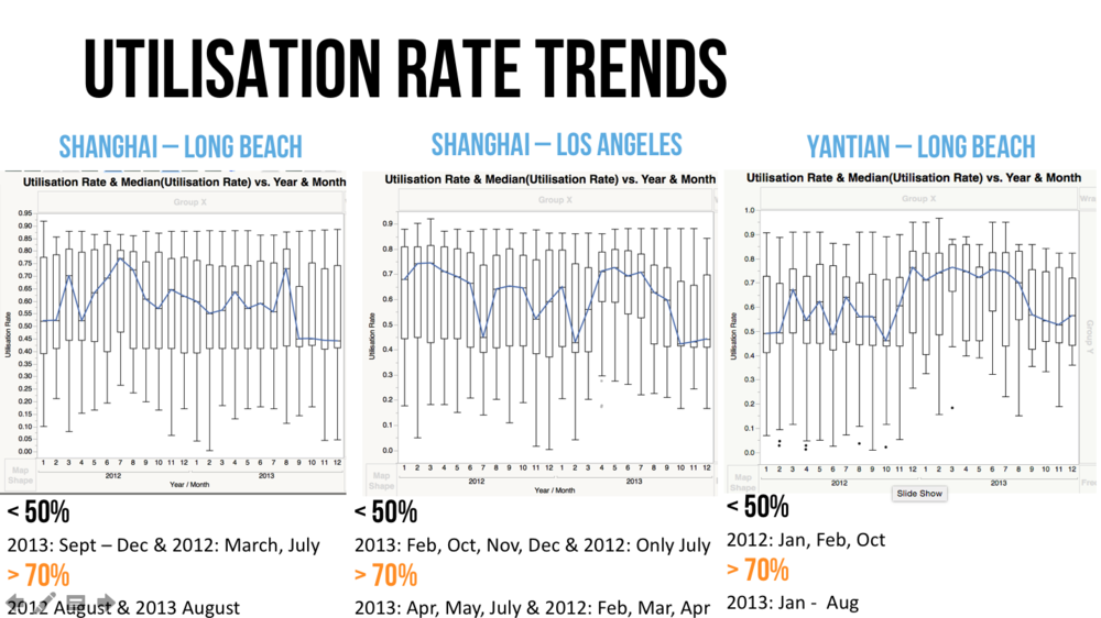
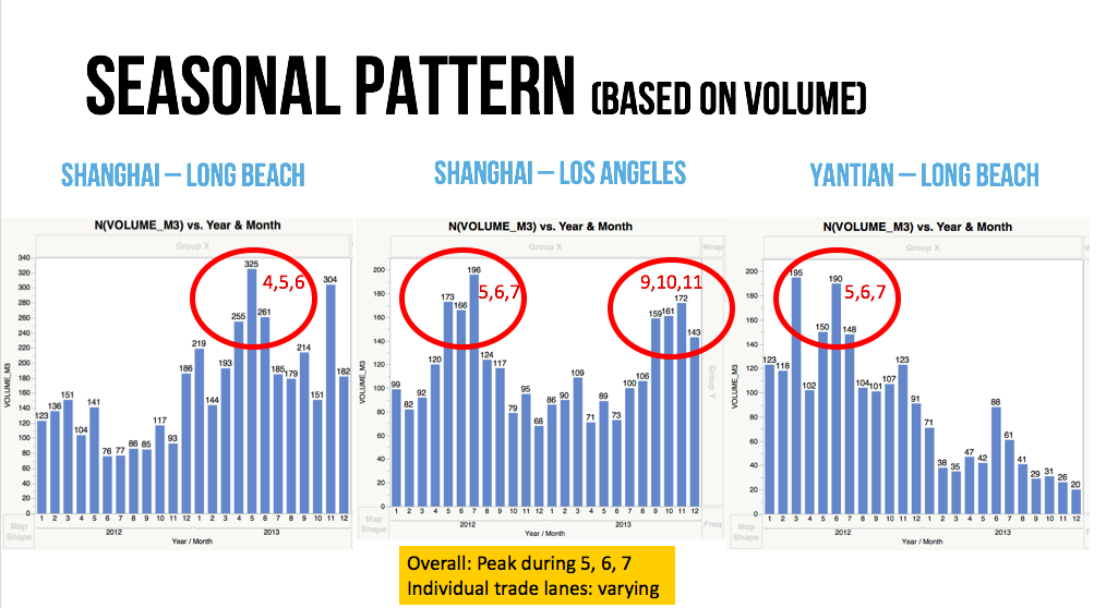
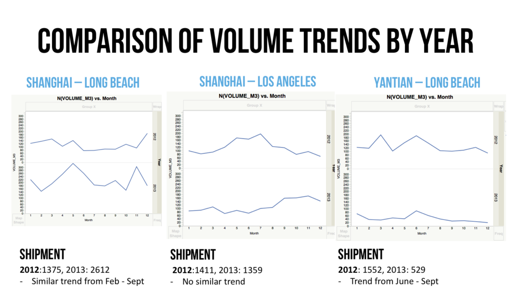
We started out by comparing the utilisation rate of the three trade lanes, followed by the seasonal patterns and volume trends.
In-depth Analysis
Building on the differences of the trade lanes, we proceeded to carry out in-depth analysis based on individual trade lanes.
For the 3 trade lanes we will be analysis, we carried out our analysis as shown below: (Example: Shanghai - Long Beach)
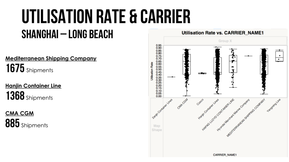
One of the major factor that affects the utilisation rate would be the type of carrier that the shipment was carried out. In the field of container shipping where the container sizes are standardised, there are yet high varying utilisation rates for the different carriers even for similar months. By looking into this factor, it allows an understanding of the type of carrier to engage in for shipments. The analysis was focused on the differences across different carriers when different factors are included, such as month, year, number of shipments, actual TEU and type of container sizes. Hence, we filtered out the carriers to see the distribution for Shanghai - Long Beach.
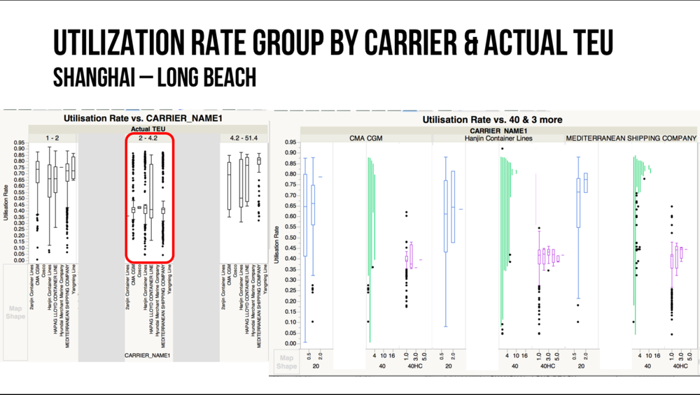
In order to provide a better in-depth analysis, we then went on to group it based on Actual TEU. Actual TEU is the unit of the capacity of a container ship, a container terminal and the statistics of the container transit in a pot. By grouping it in this manner, we are able to further classify the performance of the carrier based on utilization rate in each TEU group.
This diagram groups Actual TEU accordingly to 1-2, 2-4.2 and 4.2 – 51.4 respectively. Within the 1 – 2 Actual TEU group, it represents that containers of size 20 feet or 40 feet as 20 feet has a TEU value of 1.0 and 40 feet has a TEU value of 2.0. As we can see, the utilization rate is consistently above 60%.
While in the group of 2 – 4.2, it consist of a combination of 20 feet, 40 feet and 40 High Cube (HC) feet containers. 40 HC feet containers have a TEU value of 2.2. From the above highlighted portion in red, it is represented that the utilization for all carriers are doing badly at a utilization rate of below 50%. This is a very intriguing phenomenon that is visible across all trade lanes.
In order to provide a better visualization of the overall distribution based on utilization rate for each carrier, we then grouped it accordingly to container size. (Refer to diagram on the right)
This would allow us to view the performance of each individual carrier. We have initially identified that Hanjin Container line has a significantly lower utilization rate of 45%. However further analysis from the above diagram shows that their 20 feet and 40 feet containers are performing equally well as compared to the other two carrier lines. The only prominent difference is that Hanjin has more 40 HC feet containers as compared to the other two carriers hence pulling down its overall utilization rate. In addition, we are also able to notice that generally 40 HC feet containers drastically lower the utilization rate to an average of 40% across all three carriers.
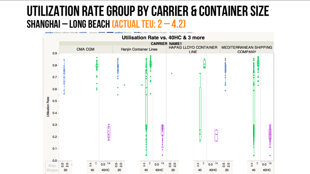
In order to understand the special phenomenon that is occurring across all trade lanes, we then performed a further analysis on this particular group. The figure above shows the distribution of the carrier based on utilization rate. As shown, the utilization rate is broken down into two groups across all carriers, above 50% and below 30%. Using the similar approach, by grouping them into container size, we are able to identify which are the main factors affecting the utilization rate in this specific group.
Significantly we are able to prove that 40 HC feet containers is the main causation across all carriers. Through the figure above, we are also able to establish that CMA CGM is doing better as compared to the other carrier in the areas of 40 feet containers within this group.
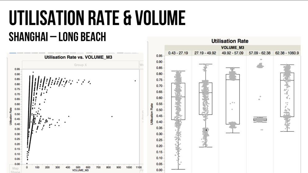
Volume is another important and crucial factor that influence utilization rate of ocean frieght. This is typically so as companies would definitely want to have a high utilization rate so as to maximize the benefits of high shipments at a minimal cost. In this part, we will look into the relationship between volume and utilization rate.
The diagram above represents how utilization rate is influenced by volume. Through this, despite seeing that higher volumes have a higher utilization rate, there is no casual relationship between these two factors.
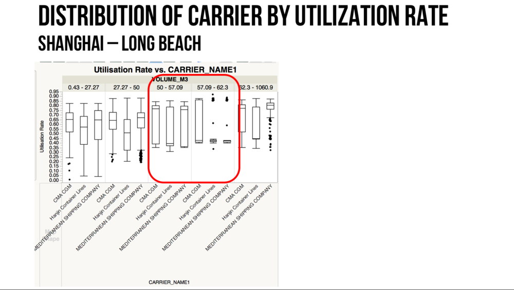
By grouping them into volume, we are now able to identify patterns within each volume percentile. As seen from the diagram, there is a very unique distribution of varying high and low utilization rate, present between the volumes of 49.92 – 57.09 and 57.09 – 62.38. This anomaly is also present in the Shanghai and Los Angeles trade lane.
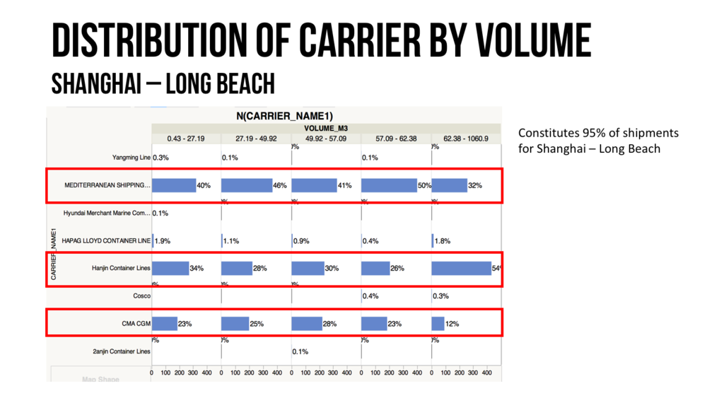
In order to fully understand the volume distribution, we went on the further classifying it based on carriers. This in turn shows the distribution of carrier based on the volume percentiles.
Correspondingly, the top three carrier lines are also distinct in this representation. This is shown in the box plots below comparing the top three carriers with utilization rate group by the volume percentiles.
Distinctively, we are able to see that Hanjin has a low utilization rate while the other two carrier has a high utilization rate of 80% in the volume of 49.92 – 57.09. While for 57.09 – 62.3, all carriers have a very low utilization rate of 40%.
Bivariate Analysis
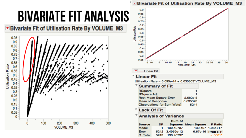
In line with all the insights between the three trade lanes, we wanted to see the relationship between these two variables, utilization rate and volume. Using a bivariate analysis, we highlighted a single portion as shown in red circle above and further tested the fit of the variables.
From above, we have established that utilization rate has a perfect RSquare correlation of 1 with volume. With this, we suspect that Volume and VolumeGDline are derived values instead of complete volumes reflective of the actual amount of volume present in the shipments. We speculate that Volume is derived from Total Volume directly.
Furthermore, the data for Total Volume seems to have variations, which are not present in Volume and VolumeGDline. This concludes that Volume and VolumeGDline are not standard values, causing it to be unable to be used in our model building.
We then went a step further to produce a best-fit line for variables of Total Volume, Actual TEU and Utilization Rate. In this analysis, we then identified that the data points for Total Volume and Actual TEU are identical hence we should only use one of the two variables for construction of our model. Similarly, by analyzing the distribution of the Gross Weight variable shows better spread of the data. Hence Gross Weight is a more suitable and appropriate variable to be used for our explanatory model.
Explanatory Model
By building an explantory model, it provides a comprehensive explanation of our data based on the insights discovered above. It seeks to explain the phenonmenon as well as the factors mainly affecting the trade lanes.
As the individual trade lanes have largely varying deviations based on characteristics as mentioned above, there is no one suitable solution model to suit all three trade lanes. Hence it is essential to build individual explanatory models.
Our main methodology used in our explanatory model is least square regression as well as stepwise regression. Stepwise regression is a semi-automated process of building a model by successively adding or removing variables based on the t-statistics of their estimated coefficients. This would result in a better model as stepwise regression would eliminate varibales that are not statistically significant hence resulting in a more accurate model.
Much as stepwise regression is said to be a-theoretical and prone to massive conceptual flaws, stepwise regression was selected as there are generally not as much literature found in terms of the aspect of selection of terms for predicting utilisation rate. Backward method is selected for stepwise regression.
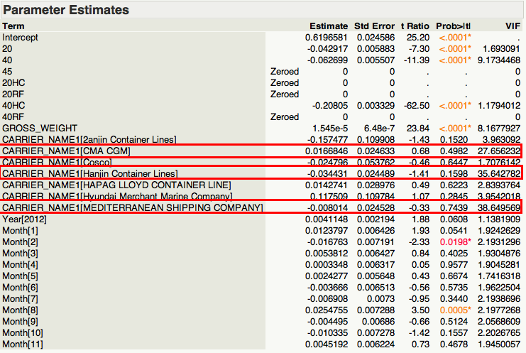
Mutlicollinearity occurs when the model containes mutiple factors that are correlated not just to the response variable but also to each other. Hence, in the case where the Variance Inflation Factor (VIF) is lesser than 1, there is no multicollinearity among the factors. The predictors may be moderately correlated in cases where VIF is more than 1. For VIF above 10, it indicates high correlation and may need to be removed from our model. (Martz, 2013)
Focusing on the parameter estimates, Carriers CMA CGM, Hanjin Container Lines and Mediterranean Shipping Company have VIF value of more than 10. Therefore, we re-run the regression model with these variables removed.
Using Stepwise Regression, the above equation signifies the main variables affecting the Shanghai – Long Beach trade lane. We then went on to profile the variables highlighting the elasticity of each of them as shown in the diagram below
From this, we are able to see 40FT containers, 40HC containers and Gross Weight has a very high elasticity. This simply means that a small change in these varibales will cause a large effect on the utilization rate. However as 40FT and 40HC containers have an inverse relationship, it is noted that an increase in either of the containers will have a decrease in Utilization Rate.
Conclusion
This paper has disccused how the analysis of an individual trade lanes can be used as an approach to build a model to improve the fill rate efficiency.
We have looked at different aspects by first doing an overview analysis based on seasonal patterns and comparison of volume trends, then an in-depth analysis on the utilisation rate against volume and the carriers used, respectively. Afterwhich, we built a bivarate model to find out the relationships between variables that were significant in influencing the utilisation rate. Lastly, an explantory model was built. As it can be seen from the results that these trade lanes have very differing patterns, a generic model is thus not feasible. Also, based on the data available, we are unable to build a predictive model.
However, with the explanatory model, we are thus able to provide to our sponsors the different factors that affect each individual trade lane, and therefore provide them with better decision-making in improving the utilisation rate. It can be done by making adjustments such as type of carriers used and container sizes for the trade lanes.
