ANLY482 AY2017-18T2 Group08 : Project Findings / Final

Homepage

Our Team

Project Overview

Project Findings

Project Management

Documentation

Other AY2017-18 T2 Projects

Interim

Final

1.0 Introduction and Project Background

In today’s world, the convenient ad-hoc access provided by digital systems is taking the place of the assured access once offered by personal ownership (The Economist, 2017). For instance, streaming beats records, cloud-system beats hard disk; credit beats cash. A similar phenomenon is occurring in the transportation industry, with the introduction of bike-sharing. Bike-sharing programs have existed for almost 50 years, but in the last decade, there has been a sharp increase in both their prevalence and popularity worldwide (Fishman, Elliot, Washington, Simon, & Haworth, 2013). Bike-sharing is a sustainable mobility strategy developed in response to concerns regarding global climate change, energy security and unstable fuel prices (Shaheen, Guzman & Zhang, 2010). Although China is currently the world leader in bike-sharing schemes, it is observed that many countries including France, Europe and USA have begun adopting this model as well (Gray, 2017).

However, despite the good and convenience that bike-sharing have introduced, there have also been downsides to it. For instance, complaints of reckless riding and bad parking have stuck a wrench in the bike-sharing movement (Lim, 2017). Authorities had little choice but to step in and issue new regulations to minimise the “bad behaviour” common among bike-sharing users.

1.1 Motivations and Objectives
Majority of existing research surrounding the bike-sharing movement consists of studies conducted with two goals in mind:
1. Understanding business profitability and sustainability concerns
2. Gathering insights on bicycle routes taken by individuals to offer guidance to urban planners, policy makers and transportation practitioners

Little or no research has yet been done to shed light on the increasingly prominent issue of illegal parking patterns. Henceforth, this paper seeks to explore this further with the following objectives in mind:
1. Fill existing research gap by exploring the use of ‘Spatial Point Pattern Analysis’ in analyzing clustering patterns of illegal bike-parking
2. Specifically demonstrate the use of KDE and modified-L-function
3. Apply the tools to a real-life case study tools based on a case study of Singapore
4. Discuss key learning points and considerations in using the methods

2.0 Literature Review

Literatures on Kernel Density Estimation (KDE) and L-function were explored and reviewed in preparation of this research. Existing literatures showed that KDE is well-suited for analyzing spatial patterns, especially when there is a need to examine the intensity of a particular phenomenon. In the paper “Spatial distribution of diagnosed chronic kidney disease (CKD) in Edo State, Nigeria”, KDE was used to investigate spatial distribution of CKD across regions in Nigeria. The study was important because health outcomes generally involve people, thus the population at risk of CKD had to be determined. Studying the spatial patterns reflects the spatial distribution of the underlying population (Carlos et al. 2010), thus allowing the team to zero into the identified regions through the use of KDE. In relation to this paper, KDE will also be adopted in identifying locations with high intensity of clustering.

The second paper “The Utility of Hotspot Mapping for Predicting Spatial Patterns of Crime” presented the usefulness and accuracy of KDE in predictive SPPA. It compared various mapping techniques such as point-mapping, thematic-mapping of geographic areas (e.g. census areas), spatial ellipses and KDE, and identifies the one that most accurately predicts future crime occurrences (Chainey et al., 2008a). It split ‘crimes’ into four categories, after-which the different techniques were applied on them to identify the technique that best predicted future crime occurrence. It was found that KDE consistently outperformed all other techniques in its predictive capabilities for all the different crime types studied. Also, data used in this paper were geocoded crime data-points, in which coordinates were rounded off to the nearest 10m. This supposedly reduces the accuracy of the data-points as a crime could have been displaced by up to 5m in any direction of the actual location. However, it was concluded that small differences in locations of crime occurrence would not negatively impact the study’s findings. This is a useful for our paper as it illustrates that research of this nature should not be sensitive to small inaccuracies of the geographical coordinates used.

Some literatures also highlighted certain inherent limitations, one of which is that KDE is unable to show the distance where spatial patterns become significant. The paper, “Identification of hazardous road locations of traffic accidents by means of KDE and cluster significance evaluation”, explored the use of KDE in determining areas with a high potential of road traffic accidents. More importantly, it also introduced the ‘Monte-Carlo Simulation’, a statistical technique that uses repeated random simulations to determine properties of event and their significance level. By combining both techniques, it allowed the researcher to identify the clusters of traffic accident that are statistically significant. Thus, to ensure the accuracy of our study, the L-function and ‘bw.diggle’, a function in R studio’s ‘spatstat’ package will be introduced to determine an appropriate kernel size for the KDE analysis. In addition, the Monte-Carlo Simluation will be adopted to ensure that the kernel size is statistically significant. More will be discussed in the next section.

3.0 Spatial Point Pattern Analysis Methods

3.1 Kernel Density Estimation

3.1.1 Origin of Kernel Density Estimation
Kernel Density Estimation (KDE), also known as the Parzen-Rosenblatt window method is a well-known approaches to estimate the underlying probability density function of a dataset (Zambom, 2012). KDE was originally used to evaluate histograms (Levine 2004; Silverman 1986), but was adapted to analyse spatial distributions (Spencer & Angeles, 2007). Since then, it has been an important method adopted by many for mapping spatial patterns of point events (Xun Shi, 2010). Some of its uses include applications in ecology (Worton 1989, Brunsdon 1995), public health and epidemiology and many other fields.

3.1.2 The Kernel Density Estimation Function
KDE is a non-parametric statistical modeling method that does not use parametric probability density functions, but only uses given data to create a statistical model (Kang, Noh & Lim, 2017). In other words, KDE automatically learns the shape of the density from a given dataset. This flexibility arising from its nonparametric nature makes it a very popular approach for data drawn from a complicated distribution (Chen, 2017).

A KDE function is obtained by combining kernel-functions generated by each value. The KDE function is defined as follows (Silverman, 1986):

K is a kernel density function satisfying ∫_(-∞)^(+∞)▒〖K(x)dx 〗=1 while h is a positive value and named as a bandwidth or smoothing parameter of the kernel-function.

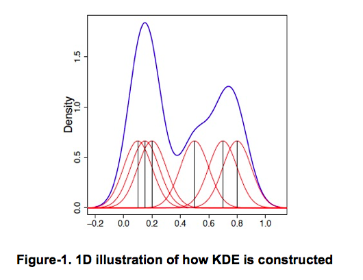
Intuitively, KDE has the effect of smoothing out each data point into a smooth bump, whose shape is determined by the kernel-function K(x). It then sums over all these bumps to obtain a density estimator. KDE yields a large value at regions with many observations, because there will be many bumps around, The converse is also true i.e. for regions with only a few observations, the density value from summing over the bumps is low.

Diagrammatically, KDE can be illustrated using a 1D-model (Chen, 2017) as shown in Figure-1 below:

3.1.3 Hotspot Mapping Using Kernel Density Estimation Function
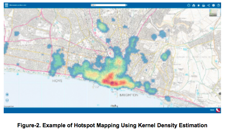
KDE is a more sophisticated representation of the services and population, where it takes the value of the data assigned to a specific point and spreads it across a predefined area. Unlike point mapping which uses discrete points, hotspot mapping focuses on continuous points and highlights areas with higher than average incidence of events, also known as ‘hotspots’. Thus, KDE has become a valuable technique for visualising geographic incidence of events and used in hotspot mapping (Figure-2). Such analysis can be implemented on geospatial softwares such as QGIS.

3.2 Ripley's K Function

Ripley’s K-function is a tool used for analysing completely mapped spatial point pattern data, i.e. data on the locations of all events within a predefined study area (Dixon 2002). Typical uses of this function include the identification of spatial patterns that occur in a data set. Real-world applications of Ripley’s K-function include the identification of clustering of proteins in membrane microdomains (Kiskowshi, Hancock, Kenworthy, 2009), spatial patterns of trees (Lin, Shi, Huang, Wan, n.d) and spatial patterns of disease cases (PJ, AG, 1991).

Ripley’s K-function formula is denoted by:

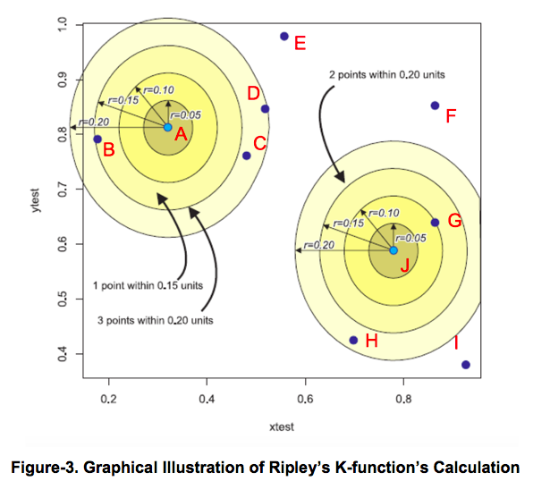
Figure-3 below is a graphical illustration of how Ripley’s K-function is calculated. Events are represented by the letters A, B, … J in the diagram below. For each event, circles of radius r are constructed around it and the number of events that fall within this radius is summed up. For instance, using A as a reference point it is observed that events B, C and D fall within the radius of r = 0.20 i.e. point A has a total count of three events within radius 0.20.

The above steps are repeated for every event in a given data set, and K(r) can be obtained by summing the results.

3.2.1 Interpretation of Ripley's K Function

The simplest use of Ripley’s K-function is to test complete spatial randomness i.e. where points events occur within a given study area in a completely random fashion (Dixon, 2001). With the assumption of complete spatial randomnessThe (CSR), the expected number of events within distance rh of each event is given by K(r) = 〖πr〗^2. If K(r) < 〖πr〗^2, the events are regulardispersed; ot. Otherwise, they are clustered.

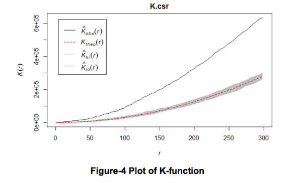
NextS, small increments of rh are made and the calculation is repeated multiple times to obtain a plot of incremental distancces/radius (r) against K(r) as shown in the figure below.

Referring to Figure-4 above, the red line indicates a plot of the theoretical line which is the expected number of events within distance r of each event in the predefined study area. The black line represents the observed line, which illustrates a plot of the actual number of events within the distance h of each focal event.

Next, the Monte-Carlo simulation test of complete spatial randomness (CSR) is used to examine whether the observed clustering is statistically significant. This is done by performing ‘M’ different independent simulations of the ‘N’ events in the predefined study area. An envelope represented by the grey area in Figure-4, can then be plotted to illustrate the distance/radius from each event where clustering become significant.

3.3 L-Function: Derivative of Ripley's K Function
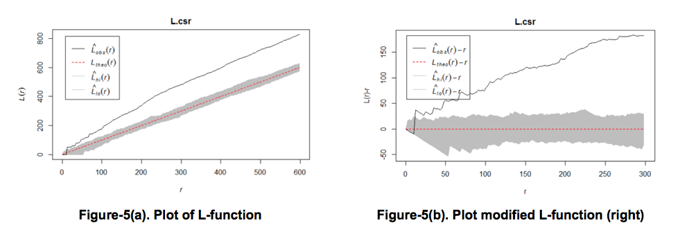
The K-function can be normalised to obtain the L-function. The L-function is more commonly used because L(r) is approximately constant under CSR (Dixon, 2002), making it easier to compare the theoretical line with the observed line. It can be further improved to obtain a modified L-function plot, L(r) - r as shown in Figure-5(b). The modified L-function sets the theoretical line to 0 for all values of r. As long as L(r) > 0, clustering of events is present. L(r) < 0 represents dispersion of events, while L(r) = 0 indicates CSR.

3.4 'Bw.Diggle' Function, An Alternative Method To Approximate A Kernel Bandwidth

The bandwidth (h) that is chosen for KDE is very important, even more so than the Kernel-function (K), in affecting the behavior of the KDE. Too small a value of h would result in too many bumps, hence resulting in false features being show. The converse would result in an estimate that is too smooth and biased, thus not revealing structural features in the data (Turlach, 1999). Although the L-function is able to determine a statistically significant bandwidth, it is an inefficient method as it runs on a ‘n x n’ matrix. Thus, researchers adopt the use of the ‘bw.diggle’ function to approximate a bandwidth for KDE analysis. This function makes use of the method by Berman and Diggle (1989) in the selection of an appropriate bandwidth for the kernel estimator. This method computes the quantity:

as a function of the bandwidth (σ).

MSE(σ) refers to the ‘mean squared error’ at each bandwidth. λ is the mean intensity, which refers to the mean number of points per unit area in the 2-D space. Lastly ‘g’ refers to the pair correction function which takes into consideration that when the distance from each event increases to a certain point, the probability of finding two events at a given distance apart from each other is approximately constant rather than continue to increase. The optimal bandwidth (σ) chosen is the bandwidth that minimizes MSE(σ). An illustration of how the optimal bandwidth is derived using this method is as follows.

This example uses a bandwidth of 1m for illustration purposes. Referring to Fgure-6, events in a study area is denoted by red dots. Take event C, there are a total of three other events within a 1m distance from it (events Q, R and B). This value is compared to the estimated number of events from event C using KDE. The MSE can be obtained by squaring the difference between the two values. This process is repeated for different bandwidths, and the bandwidth where the MSE is minimized is selected as the optimal bandwidth for KDE.

4.0 Case Study of Singapore and a Bike-sharing Firm

As a dense urban city with a growing tech-savvy population, Singapore is well-suited to adopt bike-sharing as an alternative to the traditional means of transportation. As such, it is not surprising that bike-sharing firms have seized the business opportunity to setup their operations there. To demonstrate the use of L-function and KDE, Singapore was selected as a case study. In 2017, three bike-sharing firms entered the Singaporean market with 1,000 bicycles. This number rose immensely to 14,000 within a year. A consequence of this high usage was the rate of illegal parking in this small country, which consequently affected both the bike-sharing firms as well as the public. As a measure to tackle this issue, Singapore’s regulatory authorities passed a bill on March 2018 to shift the responsibility of managing the situation to bike-sharing firms. In addition to existing warnings and potential fines imposed, the number of bike licenses each company can obtain will depend heavily on its ability to respond effectively to illegal parking occurrences.

The severity of the illegal parking phenomenon, coupled with the urgent need for operators to develop a more efficient way to respond to such cases makes Singapore a good case study to explore how L-function and KDE can be used simultaneously to analyse spatial patterns of illegal bike parking, and develop insights for the bike-sharing operators. To facilitate the analysis, data was provided by one of the bike-sharing firms currently operating in Singapore.

4.1 Dataset Description

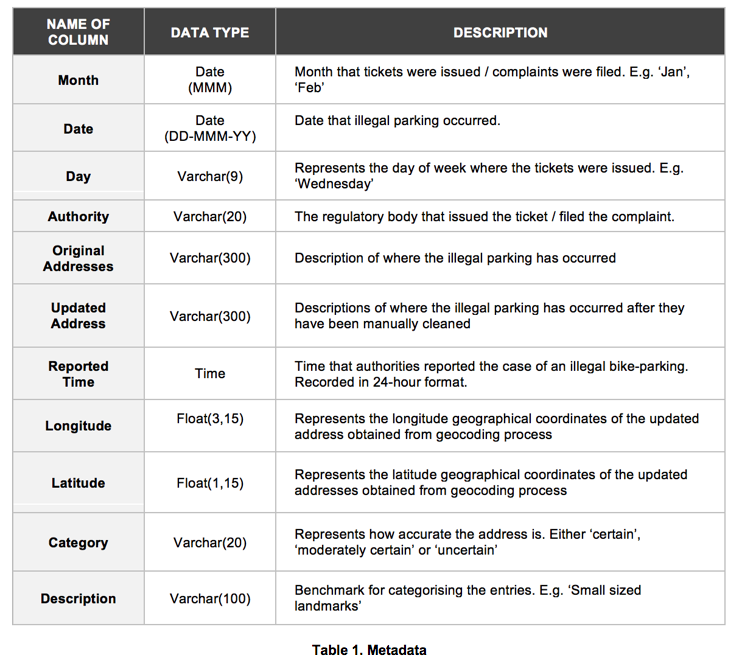
A total of 10,230 unique data points containing addresses of illegal parking were provided for this case study. The table below shows the metadata provided.

4.1.1 Geocoding Process
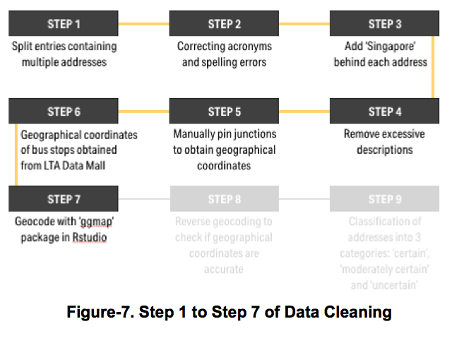
A geocoding data preparation step was necessary to transform the ‘Original addresses’ in the dataset to geographical coordinates i.e. longitude and latitudes. The following steps were undertaken in this data cleaning and preparation process:

Data Cleaning I. Entries with multiple locations were split up into separate entries to denote different illegal parking occurrences II. Acronyms and spelling errors were corrected and replaced with their actual names (e.g. ECP to East Coast Park) III. ‘Singapore’ was concatenated to all entries to restrict coordinates to Singapore’s boundary IV. Excessive descriptions not recognised by ‘ggmap’ were removed

Data Preparation V. The geocoding process was conducted in the ‘R-studio’ with the use of the ‘ggmap’, a spatial visualization package, and the Singapore Land Transport Authority (LTA) data mall. Using the cleaned data file, every row or ‘address’ was passed to Google's API and returned with their respective coordinates VI. Junctions were manually pinned on Google Maps to obtain more precise coordinates

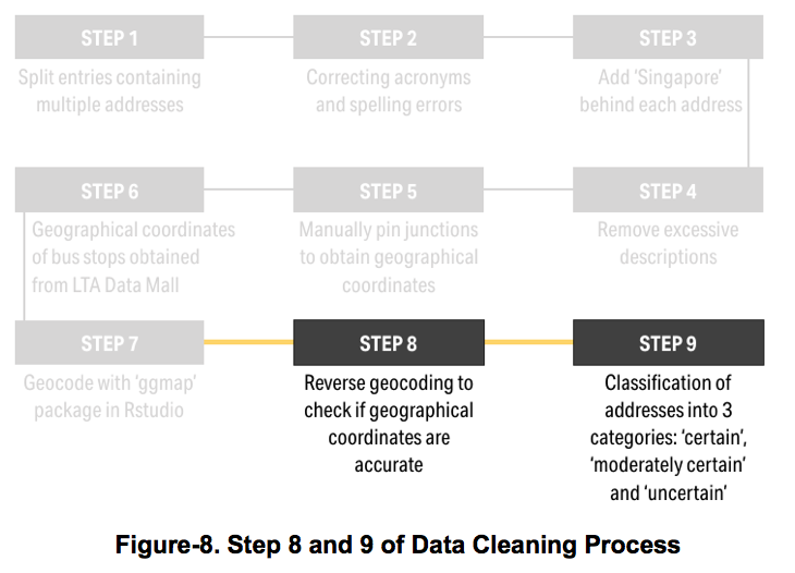
4.1.2 Classification of Locations Based on Certainty Level

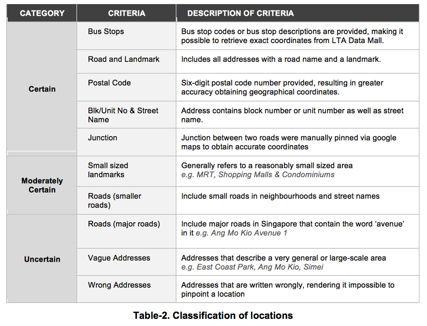
Data cleaning presented a pressing problem i.e. several addresses provided were recorded wrongly and/or vague. To obtain a rough idea about how accurate the addresses in the dataset were, the addresses were classified into the groups based on the following criteria in Table-2:

After classifying each address into the three distinct categories, it was possible to determine the accuracy of the data points. As shown in the figure below, it was observed that 6,219 (60.79%) of the entries were certain, while 1,880 (18.38%) were moderately certain. The remaining 2,131 (20.83%) points were uncertain.

As uncertain data points will result in inaccurate longitude and latitude coordinates, all 2,131 entries belonging to the ‘uncertain’ category were omitted entirely for subsequent analysis.

5.0 Application of Geo-spatial Point Pattern Analytical Methods on A Case Study of Singapore

This section demonstrates the application of geo-spatial point pattern analysis on Singapore, with the use of QGIS and R-Studio. QGIS is an open-source cross-platform desktop geographic information system application that supports various vector raster, database formats and functionalities (QGIS, n.d). It allows for creation, analysis, editing and visualization of geospatial information (QGIS, n.d).

QGIS was utilized to generate choropleth maps and heatmaps of illegal bike-parking occurrences around Singapore. A plug-in, ‘OpenStreetMap’ was also used to further enhance the visual output by providing micro details on the map. Other uses of it include the conversion of csv files into shape files and extraction of points within subzones to conduct the L-function and KDE analysis, which will be covered in the following sections.

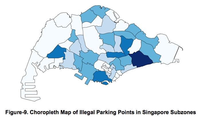
5.1 Narrowing of Study Area Using QGIS Choropleth Map To find out the number of reported illegal parking cases in each of Singapore’s subzone, a choropleth map was first generated using one of QGIS’ analysis tools – “count points in polygon”, as shown in Figure-9 below. This map provides information on the number of illegal parking cases within each subzone. The darker the shade of blue, the greater the aggregated count of illegal bike-parking cases in that area.

According to Figure-9, Bedok showed the highest collective number of warnings, with a total of count of 852 cases, followed by Jurong-West with 537 cases. However, having knowledge of the raw count is insufficient, thus further analysis has to be conducted in order to gain meaningful insights of the sub-zones.

QGIS was used to crop the Singapore subzone map and obtain independent subzones data of Bedok and Jurong-West. After which, a standardization process was performed i.e. converting all the data points which were in geographical coordinates to the Singapore Coordinate System – EPSG: 3414 SVY21. This ensures that the unit of measurement is standardized to ‘meters’. Lastly, QGIS was used to convert the files into ‘shape files format’, a format compatible with the ‘Spatial Point Pattern’ analysis on R Studio.

5.2 Determining Spatial Patterns Using Spatstat's Modified L-Function on R Studio The Modified L-Function was used to determine and analyse the spatial patterns i.e. dispersion, clustering or random occurrences of warnings issuance. This was executed using ‘R’, a language and environment for statistical computing and graphics generation on ‘R studio’, and with the support of other open-source packages, namely ‘rgdal’, ‘maptools’ and ‘spatstat’ (Table-4).

Two files, namely the ‘Bedok’s Subzone Map’ and the ‘Reported illegal bicycle parking cases’ were used to plot the Modified L-function graph for Bedok. All layers used in QGIS were in a shapefile format and the coordinate reference system (CRS) was set to SVY21. The original dataset containing geographical coordinates of illegal bike-parking cases was also converted from a ‘csv’ format to the appropriate format by QGIS.

5.2.1 Plotting The Modified L-Function Graph on 'R Studio'

Note: Only Bedok’s data and shapefiles are used in the following R-code illustration. However, Jurong-West’s analysis was still conducted in this paper.

To plot the Modified L-Function Graph, the three packages “rgdal”, “maptools” and “spatstat” had to be installed onto ‘R studio’.

Once installed, the respective shapefiles, ‘Bedok’s subzone map’ were then read into ‘R studio’ using the readOGR() function in the “rgdal” package.

The files read were then converted into the appropriate ‘ppp format’ as required by the “spatstat” package.

The ‘Bedok subzone file’ was combined with the illegal bike-parking cases ‘ppp’ file to limit the analysis to Bedok’s subzone only.

As the data was collected over three months, there were instances of repeated warnings in the same location. The presence of these duplicated data points will skew the findings and affect the accuracy of the modified L-function plot. Moreover, the purpose of the modified L-function is to determine the presence of clustering i.e. at what distance does clustering becoming significant, as opposed to identifying the intensity of clustering i.e. the number of events occurring at the same location/proximity. To ensure the accuracy of the plot, the function ‘unique()’ was used to remove all duplicated points within the data set.

A 99% confidence level was set for this study. To ensure that the results of the Modified L-function is statistically significant within this 99% confidence level, the Monte-Carlo Simulation was conducted 99 times (nsim = 99)* to generate the confidence envelope around the Modified L-function plot.

• The ’R’ syntax starts counting numerically from 0. Therefore, ‘nsim = 99’ represents a count from 0 to 99, which equates to 100 total simulation. Alpha = 1 / 100 = 0.01, thus signifying a confidence interval of 99%.

Lastly, the modified L-function graph was plotted using the “Lest” function in the spatstat package.

5.3 Obtaining the Modified L-Function PLot and Kernel Radius

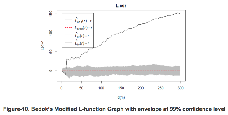
The resultant plot for illegal bike-parking in Bedok is shown in Figure-10 below.

Referring to Figure-10, it can be observed that there is significant clustering of illegal bike-parking cases at a distance of approximately 10 meters – point where the L(d)-r line exceeds the envelope.

5.3.1 Optimal Kernel Density Radius Obtained Using Spatstat's 'bw.diggle' function

The ‘bw.diggle’ function in ‘spatstat’ package was used to obtain an appropriate bandwidth that would be used in executing the KDE. It selects an appropriate bandwidth, σ, that minimises the mean squared errors as illustrated by Diggle (Diggle, 1985). The appropriate bandwidth generated through the use of this function is 96 meters as shown below.

The output of the ‘spatstat’ ‘bw.diggle’ function was an optimal kernel radius of 96m at which clustering occurs. To ensure a fair and consistent analysis, this 96m kernel size was utilized in the remaining Kernel Density Estimation analysis and QGIS heatmap plots.

6.0 Findings and Analysis

Note: Kernel radius of 96m and Pixel size of 30m is used in all analysis within this section

This section will be exploring the findings obtained from the heat maps of Bedok and Jurong-West generated on QGIS. First, a comparison is drawn between Bedok and Jurong-West to identify hotspots where warnings were issued. Subsequently, a deeper analysis on Bedok will be conducted to examine the warning issuance patterns over three distinct time periods – morning, afternoon and evening.

When we conducted our analysis with L-function and KDE on our case study of Singapore. We had a few goals in mind – firstly, we wanted to identify hotspots of illegal parking cases in Bedok and Jurong, which means we want to find out where exactly are bicycles clustering at? Is it shopping malls, schools, community centers? The second is that we wanted to validate the placement of yellow boxes – to see if we could out if the yellow boxes are indeed working. & lastly, to identify patterns of clustering with regard to time period – so we wanted to see if different timings had an effect on where the bicycles are clustering at.

6.1 Comparison of Bedok and Jurong West Using KDE on QGIS
Using the KDE plot on QGIS, the following heat maps of Bedok and Jurong-West were obtained. The scale on the right refers to the expected number of points within each kernel pixel of 30 by 30m.

It was observed that the spread of illegal bike-parking warnings in both subzones are fairly similar, where it sees a general distribution across the subzone, with a few concentrated areas denoted by the darker shade of colours. After zooming into the specific areas with high intensities, it is crucial to note that the places where the high clustering occurred for both subzones are different.

6.1.1 Bedok Subzone Heatmap Analysis
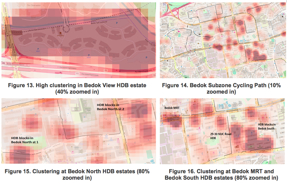
In Bedok, the HDBs are the primary areas in which high clustering of illegal bike-parking occurs, particularly in the region of Bedok North and Bedok South housing estates (Figure 13 and 15). It is notable that Bedok MRT station is also populated with illegal bike-parking occurrences (Figure-16).

6.1.2 Jurong-West Subzone Heatmap Analysis
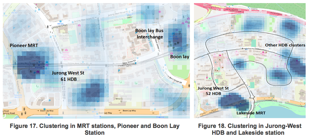
Jurong-West on the contrary sees a high level of clustering primarily at MRT stations and major cycling paths (figure-17). The secondary area of high level clustering are observed in Jurong-West’s HDB estates (figure-18).

6.2 Evaluating Placement of Yellow-boxes
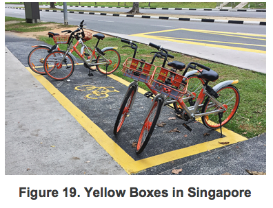
One of the measures put in place to curb the cases of illegal bike-parking is the use of ‘Yellow Boxes’. ‘Yellow boxes’ are designated parking zones specially for the bikes of these bike-sharing firms. They are marked by a physical yellow box often painted on the ground near bus-stops, MRT stations and the void deck of HDBs to prevent road obstruction (figure-19).

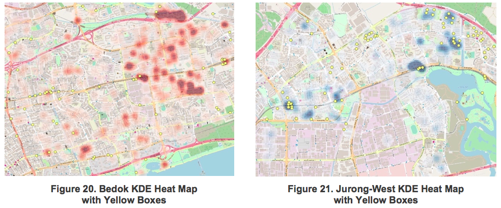
The wrong placement of ‘Yellow Boxes’ could potentially be a driver of illegal bike-parking occurrence. Building on the existing Bedok and Jurong-West heat map, a new layer containing coordinates of ‘Yellow boxes' was added on using QGIS, indicated by the yellow circles as seen in figure 20 and 21.

Referencing to figure-20, the intensity of clustering appears to be aligned with the placement of yellow boxes i.e. low occurrences of clustering in areas with yellow boxes and vice versa. For instance, there are little yellow boxes painted in the Bedok North HDB estates where high clustering of bicycles was observed. Thus, a possible solution would be to paint more yellow boxes in the void decks of the HDB estates.

A different observation is made of Jurong-West however. The yellow boxes appear to be effective in most places with the exception of the three MRT stations. There is a high level of clustering at the stations despite having multiple yellow boxes at each station.

6.3 Analysis of Illegal Bike-Parking Patterns in Bedok by Time Period
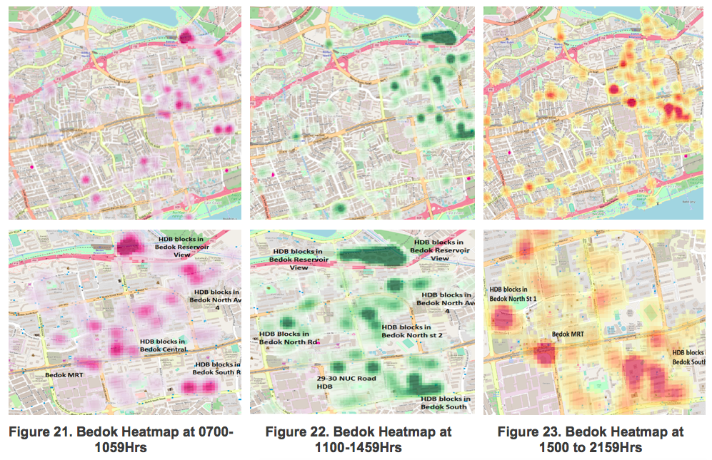
The nature and level of human traffic movement and activities tend to differ across different time period. The Bedok subzone data was broken into three different time periods, ‘0700 to 1059hr’, ‘1100 to 1459hr’ and ‘1500 to 2159hr’, after which the respective modified L-function graphs were generated.

Based on the L-function graph, it shows that clustering becomes significant at approximately 10m. Similarly, the ‘bw.diggle’ function was ran on all three datasets to generate the optimal kernel radius for analysis. The outputs were 108m, 80m and 120m respectively. To ensure a consistent comparison, the radius of 120m was kept constant in plotting all the heat maps.

Referencing Figure 21 and 23, clustering patterns and intensities are very different across the different time periods in Bedok Subzone.

6.3.1 Morning Session 0700 to 1059hrs
The highest intensity of reported illegal bike parking cases are located within the Bedok Reservoir View HDB region., whereas other areas such as Bedok MRT has a lower level of clustering. It is also notable that the clustering intensities are different across different time periods in most regions, especially near Bedok Reservoir View HDB.

6.3.2 Afternoon Session 1100 to 1459hrs
Morning and afternoon locations are largely similar with a few differences. First, clusters in the afternoon are bigger and has a greater intensity, particularly in the Bedok Reservoir View and Bedok South HDB region. Second, there is a drop in intensity around the Bedok MRT region.

6.3.3 Evening Session 1500 to 1900hrs
There is a general dip in the number of reported illegal parking cases in the evening period. Clustering is observed primarily in three areas – HDBs at Bedok North St 1, Bedok MRT and HDBs at Bedok South. At these locations, the bike firms can expect 4.24 more cases within a 30x30m radius within a 2.5-month duration of the reported case for every one illegal bike parking case reported.

7.0 Conclusion | Key Takeaways and Considerations

In conclusion, this present analysis using KDE of illegal bike-parking distribution represents an advancement in the studies involving bike-sharing. By using KDE, this study was able to analyze areas in Singapore where a greater intensity of illegal bike-parking occurs. With L-function and ‘bw.diggle’, this study has shown that illegal bike-parking in Singapore shows signs of significant clustering, and was able to determine the distance where clustering becomes significant. This value adds to the analysis by allowing a more precise input of r in KDE, as opposed to choosing an arbitrary figure.

8.0 References

Anderson, T. (2009). Kernel density estimation and K-means clustering to profile road accident hotspots. Accident Analysis and Prevention, 41(3), 359-364.

Bw.diggle function. (n.d.). Retrieved April 8, 2018, from https://www.rdocumentation.org/packages/spatstat/versions/1.55-0/topics/bw.diggle

Bíl, Andrášik, & Janoška. (2013). Identification of hazardous road locations of traffic accidents by means of kernel density estimation and cluster significance evaluation. Accident Analysis and Prevention, 55, 265-273

Chainey, S., Tompson, L., & Uhlig, S. (n.d.). The Utility of Hotspot Mapping for Predicting Spatial Patterns of Crime. Retrieved April 8, 2018, from https://www.e-education.psu.edu/geog884/sites/www.e-education.psu.edu.geog884/files/image/lesson2/Chainey et al. (2008).pdf

China's ‘Uber for bikes’ model is going global. Retrived from https://www.weforum.org/agenda/2017/06/china-leads-the-world-in-bike-sharing-and-now-its-uber-for-bikes-model-is-going-global/

Chapter 11 Point Pattern Analysis / Github https://mgimond.github.io/Spatial/point-pattern-analysis.html Diggle, Peter. (1985). A Kernel Method for Smoothing Point Process Data. Applied Statistics. 34. 138-147. 10.2307/2347366.

Dixon, Philip M., "Ripley’s K function" (2001). Statistics Preprints. 52. http://lib.dr.iastate.edu/stat_las_preprints/52

Gesler, W. (1986). The uses of spatial analysis in medical geography: A review. Social Science & Medicine, 23(10), 963-973.

Hashimoto, Yoshiki, Saeki, Mimura, Ando, & Nanba. (2016). Development and application of traffic accident density estimation models using kernel density estimation. Journal of Traffic and Transportation Engineering (English Edition), 3(3), 262-270.

Kiskowski, & Hancock, & Kenworthy. (2009, May) On the Use of Ripley's K-Function and Its Derivatives to Analyze Domain Size. Retrieved from, http://www.cell.com/biophysj/abstract/S0006-3495(09)01048-0

Kobylińska, K., Cellmer, R., Źróbek, S., & Lepkova, N. (2017). Using Kernel density estimation for modelling and simulating transaction location. International Journal of Strategic Property Management, 21(1), 29-40. Li, Wei, Huang & Ye. (2008). Spatial patterns and interspecific associations of three canopy species at different life stages in a subtropical forest, China. Retrieved from, http://www.jipb.net/tupian/2008/3/18/163001.pdf

Lim, Kenneth. (2017) Bike-sharing in Singapore: A look at the road ahead. The Channel News Asia. Retrieved from. https://www.channelnewsasia.com/news/singapore/bike-sharing-in-singapore-a-look-at-the-road-ahead-8867898

Minoiu, C., & Reddy, S. (2008). Kernel density estimation based on grouped data : The case of poverty assessment , Washington, District of Columbia : International Monetary Fund (IMF working paper ; WP/08/183).

Ripley’s K function Philip M. Dixon Volume 3, pp 1796–1803 in Encyclopedia of Environmetrics (ISBN 0471 899976) https://www3.nd.edu/~mhaenggi/ee87021/Dixon-K-Function.pdf

Silverman, B. (1978). Weak and Strong Uniform Consistency of the Kernel Estimate of a Density and its Derivatives. The Annals of Statistics, 6(1), 177-184.

Shaheen, S., Guzman, S., & Zhang, H. (2010). Bikesharing in Europe, the Americas, and Asia: Past, Present, and Future. Spencer, J., & Angeles, G. (2007). Kernel density estimation as a technique for assessing availability of health services in Nicaragua. Health Services and Outcomes Research Methodology, 7(3), 145-157.

Silverman, B.W. (2012, Mar) DENSITY ESTIMATION FOR STATISTICS AND DATA ANALYSIS B.W. Silverman. Retrieved from, https://ned.ipac.caltech.edu/level5/March02/Silverman/paper.pdf

Tania L King, Lukar E Thornton, Rebecca J Bentley, & Anne M Kavanagh. (n.d.). The Use of Kernel Density Estimation to Examine Associations between Neighborhood Destination Intensity and Walking and Physical Activity. PLoS ONE, 10(9), E0137402.

The Economist. (2017, Dec 19). How bike-sharing conquered the world. Retrieved from, https://www.economist.com/news/christmas-specials/21732701-two-wheeled-journey-anarchist-provocation-high-stakes-capitalism-how

Turlach, Berwin. (1999). Bandwidth Selection in Kernel Density Estimation: A Review. Technical Report.

Xun Shi (2010) Selection of bandwidth type and adjustment side in kernel density estimation over inhomogeneous backgrounds, International Journal of Geographical Information Science, 24:5, 643-660, DOI: 10.1080/13658810902950625

Zambom, A., & Dias, R. (2012). A Review of Kernel Density Estimation with Applications to Econometrics.

9.0 Acknowledgement

We would to graciously thank Professor Kam Tin Seong (Associate Professor of Information Systems; Senior Advisor, SIS) and Instructor Meenakshi who provided our team with great insights and guidance throughout this entire project. We would also like to thank our sponsor for graciously providing us with dataset and assistance.