ANLY482 AY2016-17 T2 Group3: PROJECT FINDINGS Cluster
| HOME | ABOUT US | PROJECT OVERVIEW | PROJECT FINDINGS | PROJECT MANAGEMENT | DOCUMENTATION | ALL PROJECTS |
Clustering Variables
After getting a clearer picture of the dataset through Exploratory Data Analysis, the next analysis that we will focus on is Cluster Analysis. The purpose of this analysis is to identify and segmentize current customers into distinct clusters of varying characteristics. First and foremost, we had to identify potential clustering variables from the Users table. After analyzing Users table, we felt that the existing variables such as age and gender was not very suitable to be used in clustering. The age range was not very wide and customers were predominantly female.
Hence, we decided to utilize the 3 variables from the RFM analysis and generate the columns shown in Figure 1 above for each customer. However, only customers with at least 1 booking were considered to ensure that the clusters formed were distinct enough. For booking_recency, it refers to the number of weeks since the customer’s last booking with respect to 31 December 2016. In terms of the monetary variable, the total monetary value of all the customer’s bookings is used instead as average monetary value is not very indicative of how much the customer had spent in the last 2 years.
Next, before commencing K-Means Clustering, it is important to understand the distribution of the 3 variables. A variable that is highly skewed will have to be normalized as K-Means Clustering is highly susceptible to such noise and outliers.
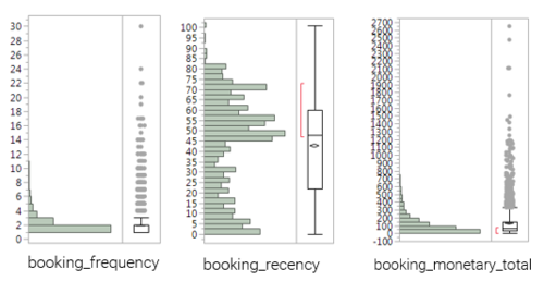
Based on Figure 2 above, booking_frequency and booking_monetary_total are highly right-skewed while booking_recency is still relatively normal. Hence, for 2 variables with a skewed distribution, a log10 transformation was used in an attempt to balance the distributions and make them more normal.
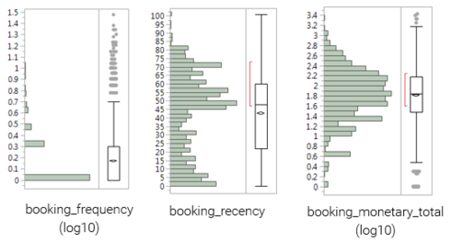
After applying the log10 transformation, the revised distributions are shown in Figure 3. Interestingly, the transformation only managed to successfully normalize the distribution of booking_monetary_total while the distribution of booking_frequency remained largely right-skewed. This was most probably due to the fact the monetary values were more continuous as compared to the frequency which seemed more discrete. Hence, we selected the initial values of booking_frequency and booking_recency as well as the transformed values of booking_monetary_total for the clustering.
Clustering Results
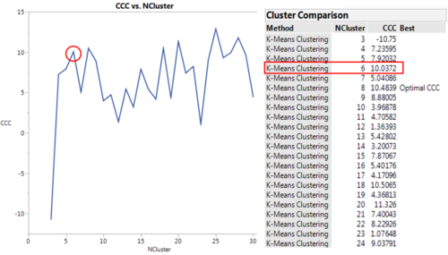
To conduct the clustering, we have utilized the in-built K-Means CLustering function found under “Multivariate Methods” in JMP Pro. However, before kickstarting the K-Means Clustering, the number of clusters had to be decided. By customizing and setting the number of clusters to range from 3 to 30, we obtained the graph shown in Figure 4 which plots the Cubic Clustering Criterion (CCC) against the number of clusters. CCC values are similar to R Squared values that basically indicate the optimal number of clusters to form. In general, the idea is to identify the point where the CCC to increase to a maximum and starts to decrease. At that point, we would then take the number of clusters as the optimal value. In this case, the optimal number of clusters to form is 6.
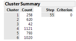
After running K-Means Clustering with and intended number of clusters set to 6, we managed to get 6 different clusters of varying counts as well as their cluster means (as seen in Figure 5 and Figure 6). At a glance, the number of customers in each cluster seem to be relatively uneven, especially in cluster 3 where there are only 42 customers present. We will look into this unique cluster and its characteristics when we profile each cluster accordingly below.
For the profiling of clusters, we have generated the Parallel Coordinate Plot for each respective cluster. This plot basically gives a more visual representation of any patterns that may arise within the cluster itself. More specifically, each clustering variable is a column with its binned range of values displayed vertically. Color-coded polylines are then drawn and the range of values the cluster contains for every variable are shown. Ideally, each cluster should have a profile that is distinct enough from other clusters.
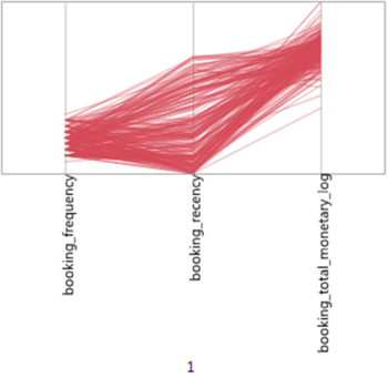
For cluster 1, the general shape of plot is relatively dense, giving the cluster distinct and unique characteristics (as shown in Figure 7). Even though this cluster only contains 258 customers, there is an average booking frequency of 6 and a decently high average total monetary value of $125. The only visible drawback is its widespread booking recency, which means that while there are customers that booked quite recently (within 1 month) there are also customers that have not booked in a while (6 months). This may imply that customers within this cluster were actually making bookings regularly and spending decently but may have stopped this behaviour in recent months.
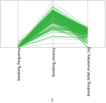
For cluster 2, the general shape of plot is also relatively dense, giving the cluster distinct and unique characteristics (as shown in Figure 8). As compared to cluster 1, this cluster has a higher number of customers (620). However, all 3 clustering variables are not too desirable where customers have only booked once, not very recently and are not willing to spend much on beauty services (average total monetary value of only $12). This seems to suggest that customers within this cluster are slowly dropping of from using the beauty application entirely.
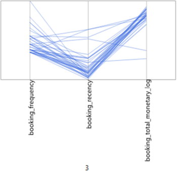
For cluster 3, as mentioned earlier, it only has 42 customers which is relatively intriguing (as shown in Figure 9). As compared to the previous 2 clusters, the shape of the cluster is understandably more sparse. However, customers within this cluster fare exceptionally well when it comes to the 3 clustering variables. There is high frequency, low recency (within 2 to 3 months) and a high average total monetary value of approximately $700. Although the number of customers within the cluster are low, this cluster could potentially represent Vanitee’s high valued group of customers that could be targeted differently.
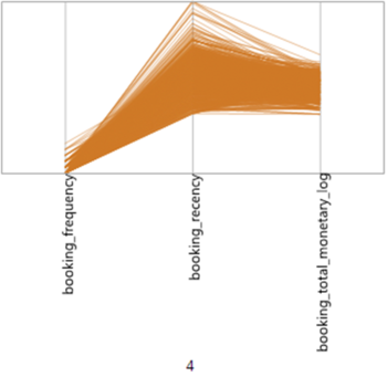
For cluster 4, the general shape of plot is also relatively dense, giving the cluster distinct and unique characteristics (as shown in Figure 10). As compared previous clusters, this cluster has a higher number of customers (1121). Unfortunately, majority of customers within this cluster have only booked once and have not booked within the last 4 months. The only upside is that they have spent an average total monetary value of $60 in their first booking which indicates that they are willing to spend but are somehow not making more bookings.
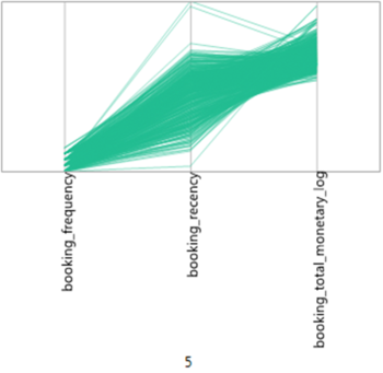
For cluster 5, the general shape of plot is also relatively dense, giving the cluster distinct and unique characteristics (as shown in Figure 11). This cluster has approximately 793 customers. Its shape is relatively similar to cluster 4 in terms of its low booking frequency. However, the booking recency of customers within this cluster is more widespread and customers are willing to spend much more on beauty services (average total monetary value of $238).
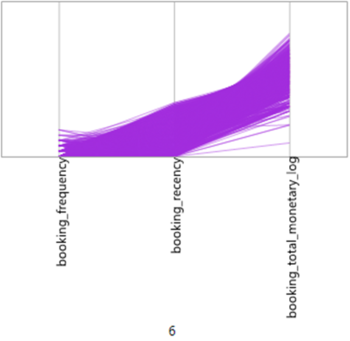
Lastly for cluster 6, the general shape of plot is also relatively dense, giving the cluster distinct and unique characteristics (as shown in Figure 12). This cluster has approximately 1020 customers. Its shape is relatively similar to clusters 4 and 5 in terms of its low booking frequency. However, the booking recency of customers within this cluster is slightly lower and customers are willing to spend a medium amount (more widespread) on beauty services (average total monetary value of $89). Clusters 4, 5 and 6 are relatively similar and may be indicate of the mass market where most customers have only booked once even though they are willing to spend on beauty services.


