ANLY482 AY2016-17 T2 Group10 Project Overview: Methodology
Contents
Tools Used
SAS JMP Pro 13 is chosen as our primary tool for data preparation, exploratory and further analysis. It is an analytical software that can perform most statistical analysis on large datasets and generate results with interactive visualizations used by data scientists to manipulate data selection on the go. Furthermore, tutorials and guides are widely available online for us to learn JMP Pro 13’s different techniques and functions.
More importantly, its easy-to-use built-in tools enable us to conduct analysis of variance to determine relationship between interactions and sales revenue.
Data Preparation
Data preparation took us through time-consuming and tedious procedures to obtain high quality data. Though seemingly unrewarding, a set of high quality data allows for more accurate, reliable and consistent analysis of results. Therefore, it is imperative to invest a lot of time and effort on it to avoid getting false conclusions for our hypothesis.
Firstly, using SAS JMP Pro, these tables are scanned for anomalies such as missing values or outliers. We corrected them appropriately, using imputation for missing values and omission for extreme outliers. This step ensures that the data we are using will not give us misleading insights.
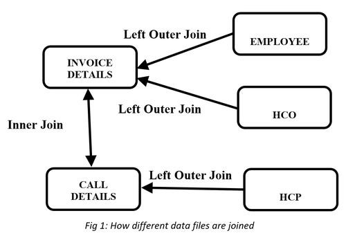
Next, to determine the causality relationship between interactions and sales revenue, we need to join Call Details and Invoice Details tables. This leads us to understand variables from both tables to find out 1) which two variables are the same and whether their formats are alike, 2) at which granularity does each row from both tables represents. Upon fully understanding them, we performed aggregations, standardizations of formats and inclusions of HCP and HCO tables to serve as links. Furthermore, we added the dimensionality of employees’ teams from Employee table, as it will be useful in describing the relationship as mentioned. Finally, we integrated relevant tables into a consolidated table and loaded it into the JMP server for analysis.
The above diagram illustrates how data tables are being integrated, which took a few stages to achieve.
Data Cleaning
The first stage of data preparation involves cleaning Invoice Details and Call Details tables.
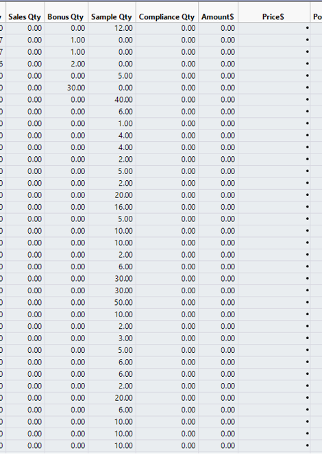
- For missing values under “price$” column in Invoice Details, we imputed their values to “0” as these rows contain records where free samples given out to customers.
- Steps Taken:
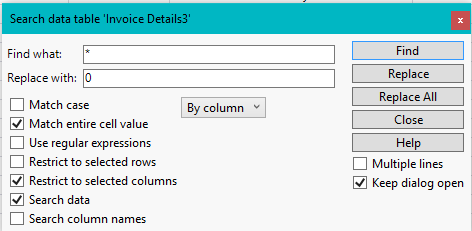
- Press Ctrl-F to show “search data tables” interface
- Steps Taken:
- Enter the following fields:
- Find what: *
- Replace with 0
- Tick “Match entire cell value”
- Tick “Restrict to selected column” of “Price$”
- Tick “Search data”
- Click on “Replace All” to apply change
- Enter the following fields:
- For negative “sales qty” and “amount$” values in Invoice Details, we did not take any action as they serve as records to void any sales that has been cancelled. Upon aggregation by quarters, no negative values will be present.
- For 5-digits postal codes in Invoice Details, we created a new column to store the converted ‘postal code’, with data type changed from numerical to categorical and formula function used to add the missing ‘0’.
- Steps Taken:
- Right click on Postal Code’s header -> Select “Column Info” -> Change data type to “Character”
- Right click on Postal Code’s header -> Select “Insert Columns”
- Right click new column -> Select “Formula” -> Enter the formula as shown below
- Steps Taken:
- Click on “OK” to apply change
- To facilitate understanding quarterly performance of sales revenue in Invoice Details and Call Details, we added a “year-quarter” column for use during aggregation.
- Steps Taken:
- Right click on “Invoice Date” of Invoice Details / “Date” of Call Details
- Select “New Formula Column” -> “Date Time” -> “Year Quarter” to create the new column
- Steps Taken:
- For “Product Names” differences in Invoice Details and Call Details, we standardized a common format using the recode function. (No screenshots due to confidentiality clause)
- Steps Taken:
- Click on “Product Name” of Invoice Details / “Product” of Call Details
- Go to “Cols” at the top -> Select “Recode”
- At the “recode” interface, input new values that are the standardized common format
- Click on “Done” and “In Place” to replace the old values
- Steps Taken:
Adding Dimensionalities
The second stage of data preparation involves adding dimensionalities to Invoice Details and Call Details tables using HCO, HCP and Employee tables.
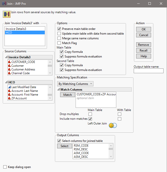
- Invoice Details and HCO are left outer joined to add dimensionality of clinic’s “name” needed for further joins, while keeping records in Invoice Details intact.
- Steps Taken:
- We have identified the matching variables to be “CUSTOMER_CODE” in Invoice Details and “ZP Account” in HCO, both are IDs of clinics
- Go to “Tables” and “Join”
- Enter fields as shown in screenshot below
- Steps Taken:
- Ensure that Left Outer Join is selected and output columns are populated before clicking “OK” to apply join
- Call Details and HCP are left outer joined to add dimensionality of “primary parent” (clinic name of individual doctors) needed for further joins, while keeping records in Call Details intact.
- Steps Taken:
- We have identified the common variables to be “Account” in Call Detailsand “Name” in HCP, both are name of doctors
- Go to “Tables” and “Join”
- Enter fields as shown in screenshot below
- Steps Taken:
- Ensure that Left Outer Join is selected and output columns are populated before clicking “OK” to apply join
- Invoice Details and Employee are left outer joined to add dimensionality of “therapy area” (sales teams) needed for further analysis, while keeping records in Call Details intact.
- Steps Taken:
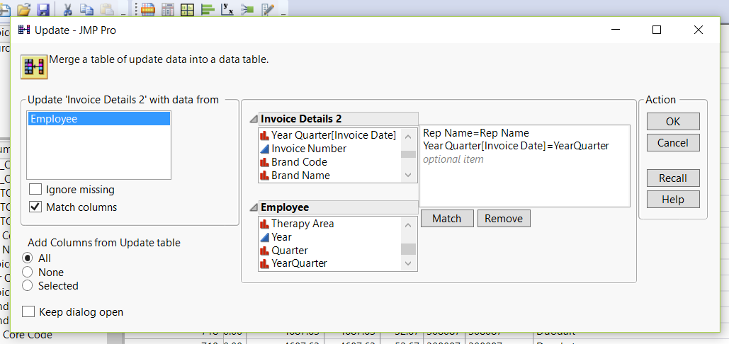
- We have identified the matching variables to be “Rep Name” in both Invoice Details and HCP, which are names of sales rep. Additionally, “year quarter” from both tables are also identified because sales reps may change their “Therapy area” (sales teams) by quarter basis.
- We will utilize another function “Update” to perform the same left outer join
- Go to “Tables” and “Update”
- Enter fields as shown in screenshot below
- Steps Taken:
- Click “OK” to apply update
Data Aggregation
The third stage of data preparation involves aggregating Invoice Details and Call Details
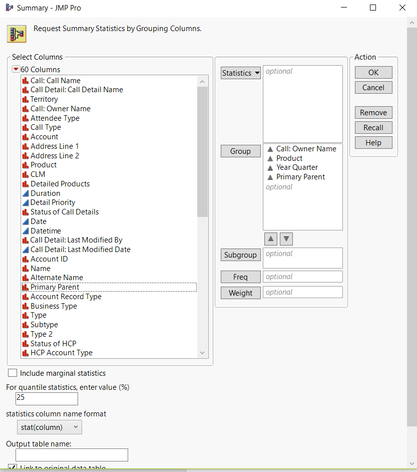
- Invoice Details are aggregated by “year-quarter” to derive additional columns “sum(sales qty)” and “sum(amount$)”, addition to variables we are interested at: “channel” (clinic type), “rep name”, “product name”, “name” (clinic’s name) and “therapy area” (sales teams).
- Steps Taken:
- Aggregation will be performed using “Summary” function.
- Go to “Tables” and “Summary”
- Drop fields to Statistics and Group as shown in screenshot below
- Steps Taken:
- Click “OK” to summarize the tables
- Call Details are aggregated by “year-quarter” and “primary parent” to derive additional column of “no. of rows” (interaction count), addition to variables we are interested at: “call: owner name” (sales rep’s name) and “product”.
- Steps Taken:
- Aggregation will be performed using “Summary” function.
- Go to “Tables” and “Summary”
- Drop fields to Statistics and Group as shown in screenshot below
- Steps Taken:
- Click “OK” to summarize the tables
Data Integration
The final stage of data preparation involves joining Invoice Details and Call Details
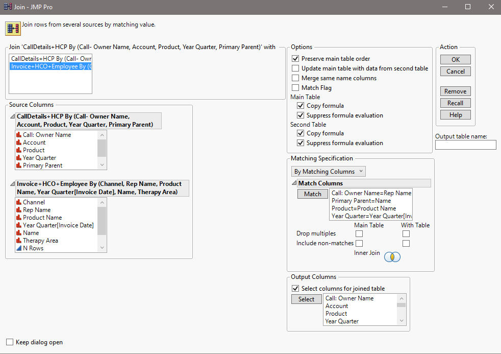
- Invoice Details and Call Details are inner joined by sales rep’s name, clinic’s name, product’s name and year-quarter. Other variables present in the final table are “channel”, “therapy area”, “interaction count”, “sum(sales qty)” and “sum(amount$).
- Steps Taken:
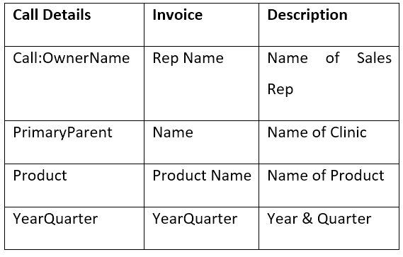
- We have identified the following matching variables from Call Details and Invoice Details
- Steps Taken:
- We will utilize Join function again to perform the inner join
- Go to “Tables” and “Join”
- Enter fields as shown in screenshot below
- Ensure that inner join is selected and output columns are populated before clicking “OK” to finish the join
ACTUAL METHOD: Analysis of Variance (ANOVA) using Fit Y by X
Analysis of Variance is a statistical method used to analyze differences among group means and their variances among and between groups. It is also a form of statistical hypothesis testing to test whether differences between pairs of group means are significant or not.
Prior to using ANOVA, we have attempted using linear regression to generalize the relationship between number of interactions and sales revenue. However, low R-squared values that suggest weak correlation and model not fitting the data were obtained, and these prompted us to carry out similar analysis using nonparametric tests like ANOVA.
The primary step to carry out ANOVA is to discretize our explanatory variable - “interaction count” into bins and as such, converting it from a numerical to categorical variable. The objective of discretization is because we wish to understand whether each of these interaction bins have significant differences between one another when it comes to sales revenue (response).
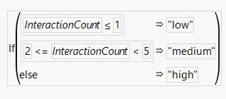
To define the range of interaction counts for “Low”, “Medium” and “High” interaction bins, we consulted our sponsor, who proposed that “Low” is for interaction count less than or equal to 1, “Medium” is for interaction count from 2 to 4 and “High” is for interaction count 5 and above.
The steps taken to discretize interaction counts into bins are as follow:
- Insert new column right of Interaction Column and name it as Interaction Bin
- Right click header of Interaction Bin, select “Formula”
- An interface to formulate the new column is displayed
- Using various Conditional and Comparison functions, enter the following formula proposed by our sponsor
- Upon clicking “OK”, the new column will be populated with values of “low”, “medium” and “high”
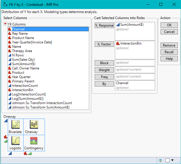
The next step to conducting ANOVA would be to use Fit Y by X function. Fit Y by X function can detect whether response or explanatory variables selected are numerical or categorical, and selectively carry out bivariate, oneway, logistic or contingency analysis. In our scenario, our “X, Factor” or explanatory variable is interaction bins (categorical) and “Y, Response” is sales amount (numerical), thus, the analysis conducted would be oneway.
The steps taken to use Fit Y by X function for ANOVA is as follows:
- Go to “Analyze” and “Fit Y by X”
- Drop Sum(Amount$) to “Y, Response” and Interaction Bin to “X, Factor”
- To look into the perspective of individual channels or therapy areas when comparing their means, we will also drop Channel or Therapy Area to “By”
- Click on “OK” to get one way analysis of Sum(Amount$) by interaction bin for individual channels/ therapy areas
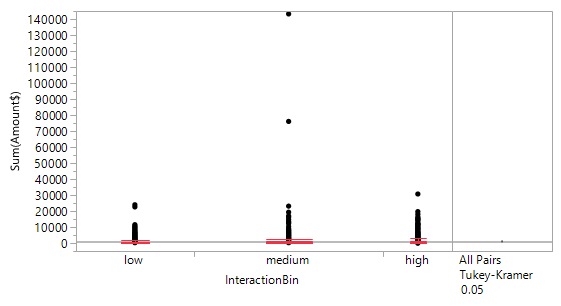
- To get in-depth details of quantiles for each interaction bin, select the upside-down red arrow and click on “Quantiles”
- Red box plot for each interaction bin will appear
- To conduct Tukey-Kramer HSD test for all pairs of interaction bins, select the upside-down red arrow again, and click on “Compare Means” and “All Pairs, Tukey HSD”
- A few reports will appear below the graph, but our attention is on the ordered differences report, which calculates p-Value to show whether differences between means of interaction bins are significant or not. Fig 16 below is an instance of the output


