ISSS608 2018-19 T1 Assign Qiao Xueyu Data Preparation
|
|
|
|
|
|
Official Air Quality Measurements
This is the official air quality data which contains 6 stations PM10 concentration from 2013-01-01 to 2018-09-14.
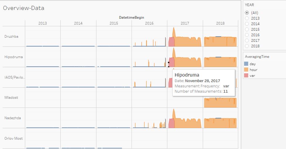
On the figure above, the height of areas represents the number of time of measurements on each day.
From this figure, we can notice that the measurement was taken hourly from 2013 to 2015, hourly on certainly days in 2016, and from 2017 onwards, the measurement was mainly taken hourly. This means we do not have hourly data from 2013 to 2016. And from the tooltip shown above, we can also notice that in 2017 the hourly data was taken only from 28 Nov, 2018 and there is no data backward 2017.
It's also worth noticing that the station of Mladost started operation only from 2018 and the station of Oriov Most stopped operation in the third quarter of 2016.
Except for the measurements from 2013 to 2018, we also have the metadata contains the information of each station including their geographical details, distance to building and curb, station types and so on. We will join the data of 6 years with the metadata in Tableau for the exploration and visualization.
Citizen Science Air Quality Measurements
The citizen science air quality measurements contain PM10 and PM2.5 concentration data measured by citizens who volunteer to collect air quality data for scientific research.
The data we have is from 2017 to 2018, and instead of longitude and latitude, the geographical information we have is geohash which is a short string representing a specific location. So to get the longitude and latitude, we need to decode the geohash first using a R library called geohash.
After encoding, we can explore the data using JMP.
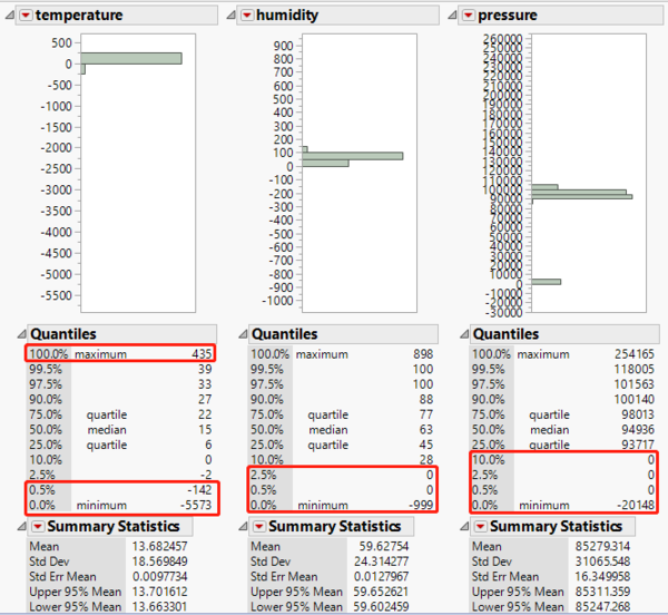
We can notice that the highest values of P1 and P2 are 2000 and 1000 respectively. Although it is possible that hourly PM10 reaches up to 1000, all the outliers come from several certain geohash codes and the readings during the same time period from other geohash codes are different from them, so we can conclude that they are anomalies due to operation issues.
Except for the abnormal reading of P1 and P2,there are also some abnormal reading of temperature, humidity and pressure.
| From the figure on the left, we can notice that there are some outliers among all the three variables. The normal temperature of Sofia is -10℃-30℃, given some of them are hourly measurement and the difference among zones, we can expand the range to -15℃-40℃ beyond which should be treated as anomalies. And since humidity is a percentage, any humidity value beyond 0-100 is anomaly including 0. And the pressure of 0 and below is also anomaly. | |
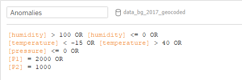
| In Tableau, we can create a calculation field as shown above to mark the anomalies for the exploration of the operations of stations. | |
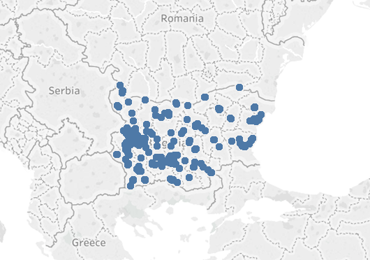
| After importing the data to Tableau, we can notice that the stations cover not only Sofia as shown below, so we need to use Lasso to incude only the dots within Sofia. |
Others
Excep for the two datasets, we also have the meteoroogical data and the topographical data, we will join them with the datasets above to explore the relationship between pollutants and other factors.
