ISSS608 2017-18 T3 Assign Akanksha Shrirang Yadav Insights
|
|
|
|
|
|
|
Analysis and Classification of Audio Files Through Visualizations
For analysis of question 2, two different approaches were implemented in order to evaluate the legitimacy of Kasios’ claim about the pipits.
- Comparison of Oscillograms of the Audio Files
- Comparison of Distribution of Plots Selected Audio Features with the Features of the Test Files
These methods were compared at the end to see if they produced similar or different results.
As the number of samples for each species is not sufficient enough, running a machine learning algorithm over such training data might yield poor results with low accuracy. Hence, in this analysis, the only focus was to do visual comparison of the plots obtained through both approaches.
Other approaches tried:
Spectrogram of all the files were plotted, but were not discernible enough for comparison of the audio files. Additionally, time measurement plots were also plotted to see if they can be useful in analysis. However, similar issue occurred while interpreting the plot. Hence, ultimately a simple oscillogram was chosen instead.
Conversion Of MP3 Audio Files to WAV
All the visualizations were built in R. As majority of the R packages can only read audio file in ‘.WAV’ format, all the audio files (All Birds & Test) were converted to ‘.WAV’ format using tuneR package.
Approach 1 - Oscillogram Comparison
- The provided audio files of all the birds have quality scores associated with them wherein the value of this score can be A, B, C, D, E or No Score. However, no description is provided about the different quality scores. For the analysis, audio files without any score were not taken into consideration.
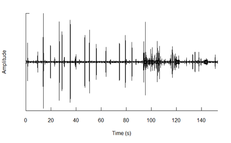
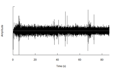
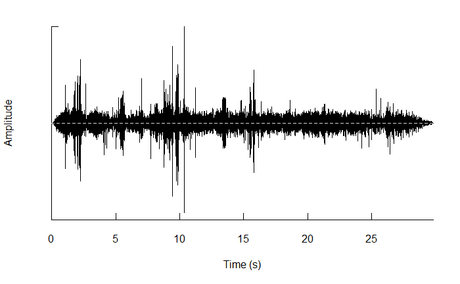
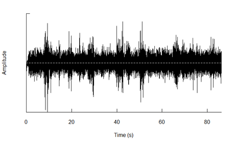
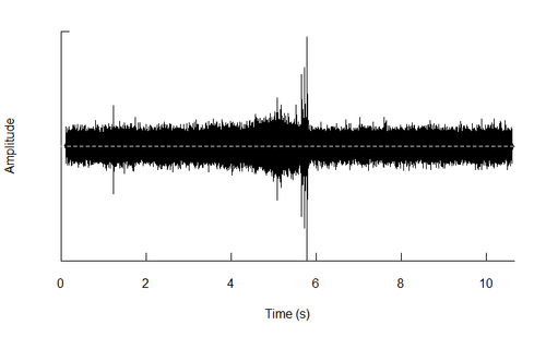
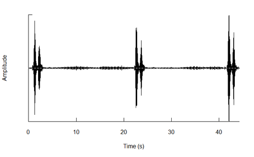
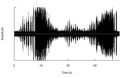
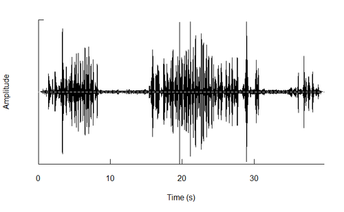
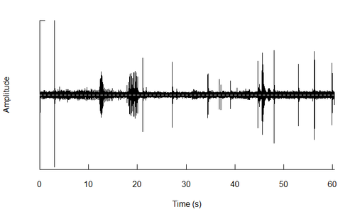
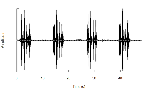
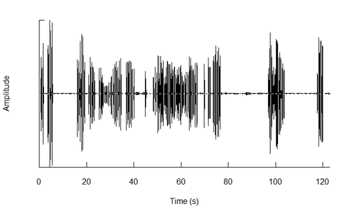
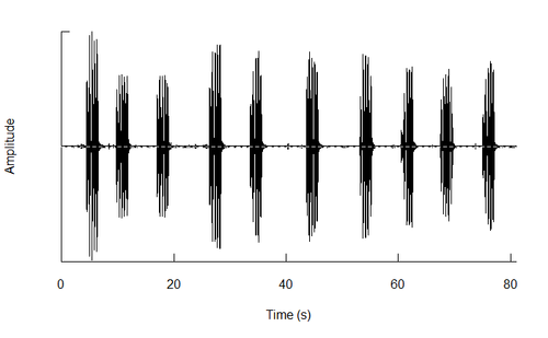
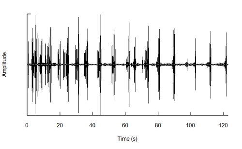
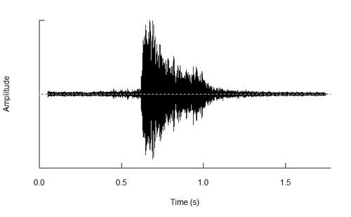
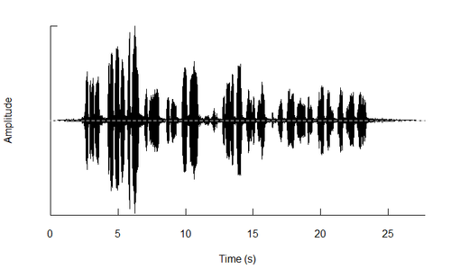
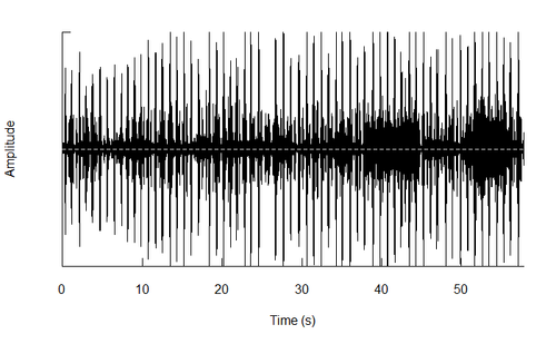
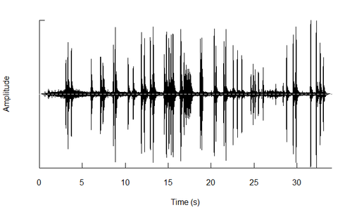
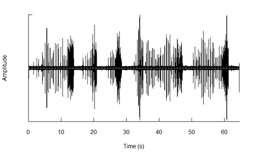
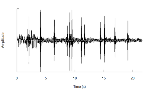
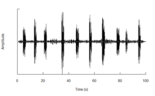
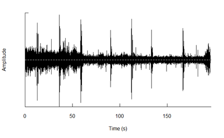
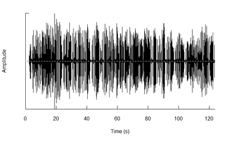
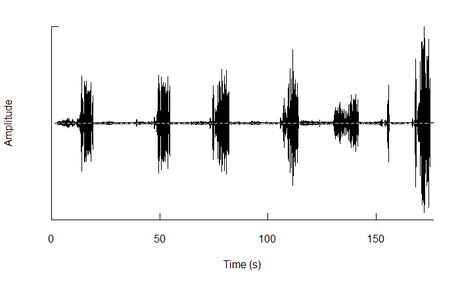
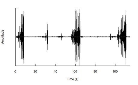
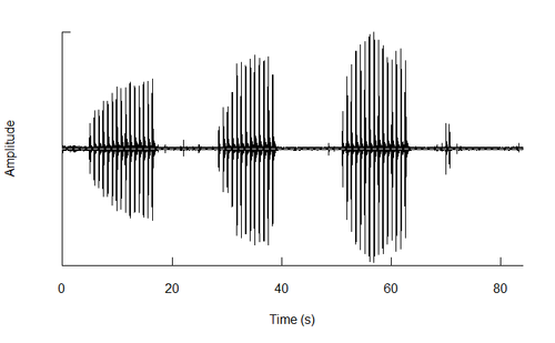
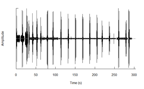
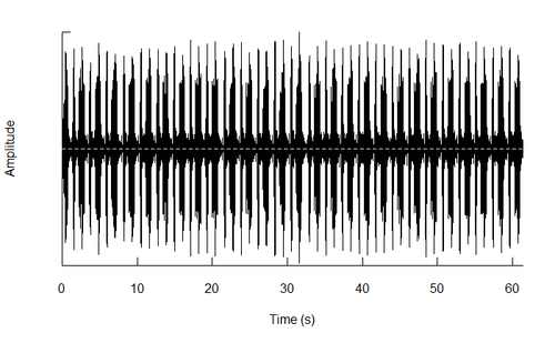
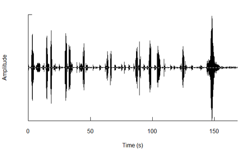
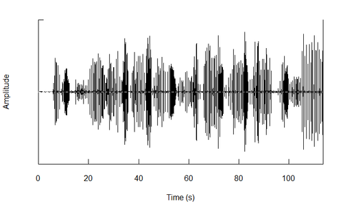
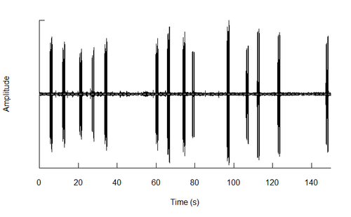
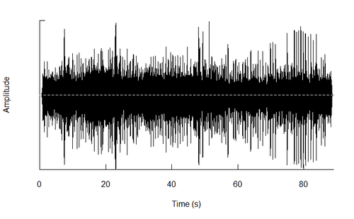
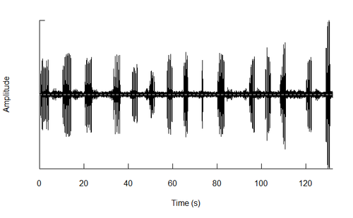
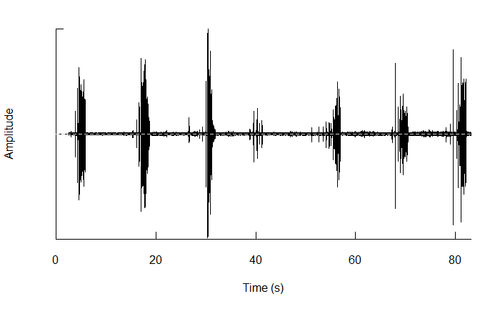
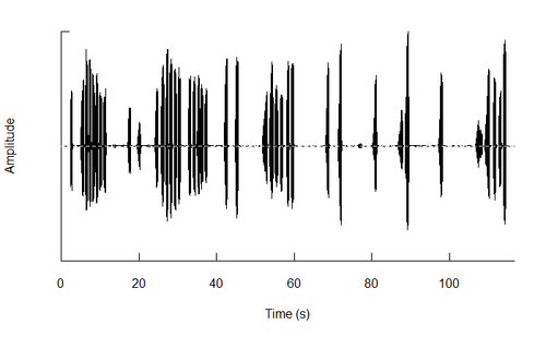
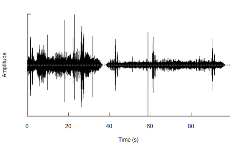
- Hence, prior to beginning with the analysis, a set of 5 files were chosen with quality scores A, B, C, D & E for “Rose-crested Blue Pipit”. Out of these 5 files, the file with score A was found to be the clearest & without much noise. All other files were found to have varying degrees of noise in them.
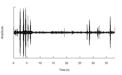
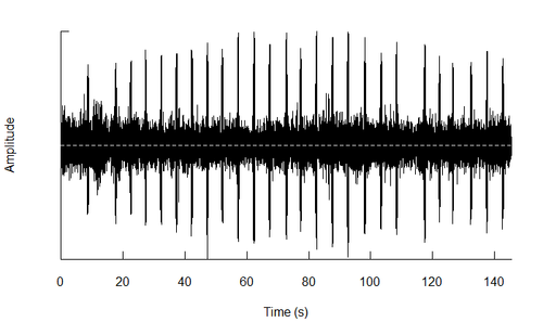
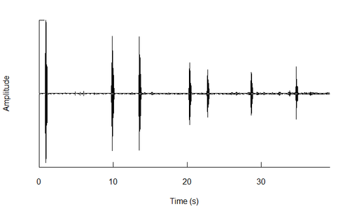
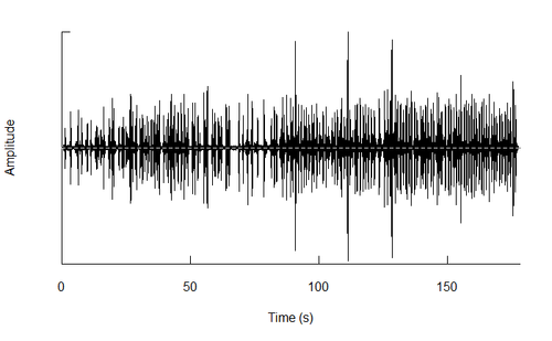
The oscillogram plots of the chosen files are as shown below:
Next, 19 training birds were chosen one from each species of the birds and their oscillograms were plotted. Similarly, oscillograms were plotted for the test files provided by Kasios. All the test plots were compared with the chosen 19 birds individually to obtain the best estimate
Now, let’s look at the oscillogram plots of 19 species of the birds:
Bent-beak Riffraff
Blue-collared Zipper
Bombadil
Broad-winged Jojo
Canadian Cootamum
Carries Champagne Pipit
Darkwing Sparrow
Eastern Corn Skeet
Green-tipped Scarlet Pipit
Lesser Birchbeere
Orange Pine Plover
Ordinary Snape
Pinkfinch
Purple Tooting Tout
Qax
Queenscoat
Rose-crested Blue Pipit
Scrawny Jay
Vermillion Trillian
The oscillogram plots of the test audio files are shown below:
Test Sample 1
Test Sample 2
Test Sample 3
Test Sample 4
Test Sample 5
Test Sample 6
Test Sample 7
Test Sample 8
Test Sample 9
Test Sample 10
Test Sample 11
Test Sample 12
Test Sample 13
Test Sample 14
Test Sample 15
Comparing the test plots obtained with train plots:
Examples are shown for a couple of the plots:
Estimated Outcome:
Approach 2 – Comparison of the Distribution Plots
For this analysis, various features of the audio files were retrieved using ‘analyzeFolder’ function found in ‘soundgen’ package in R. This function has the capability of processing batch files as well as also outputs the result in a summary dataframe which contains all the extracted features for all the files.
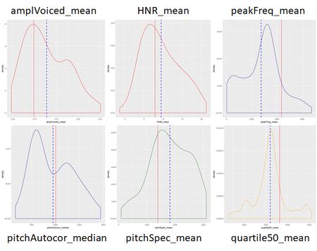
70 such features were obtained from the audio files. To reduce the number of variables, correlation plot was obtained to discard highly correlated variables. The variables were then clustered in hierarchical clusters using ‘Variable Clustering’ method in SAS JMP. Finally, the following 6 features were selected for further analysis:
<<6 variables>>
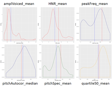
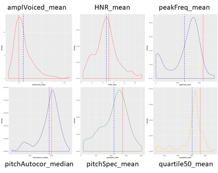
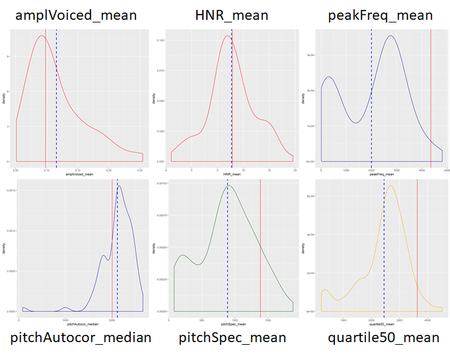
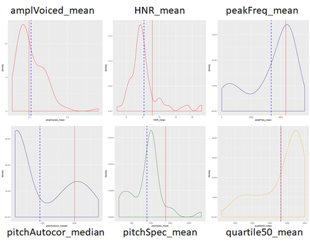
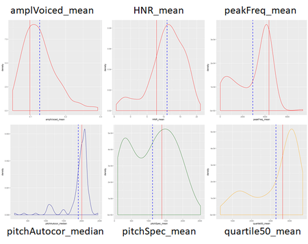
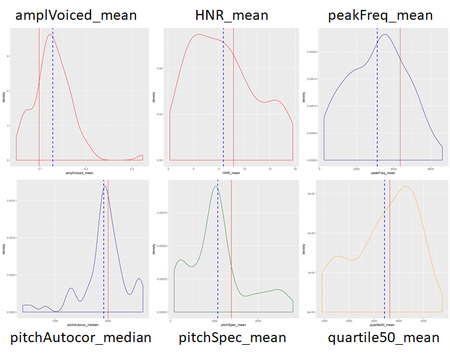
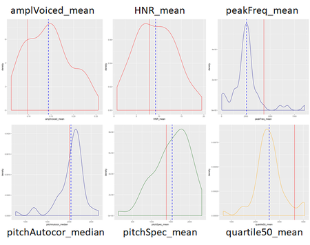
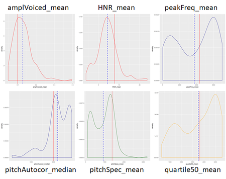
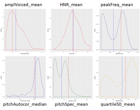
Next, the distributions for these variables for all the 19 species were plotted.
Similar features were obtained for the test audio files.
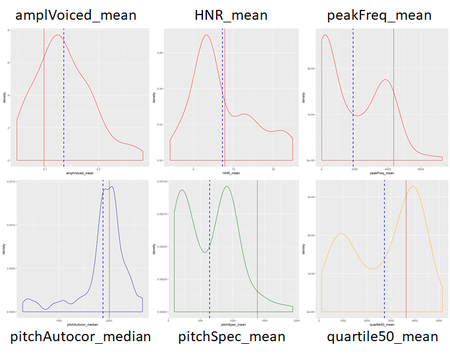
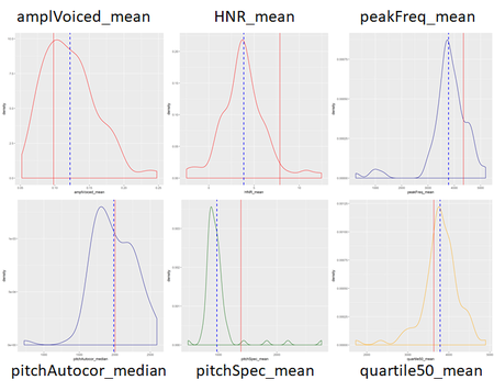
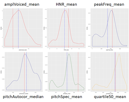
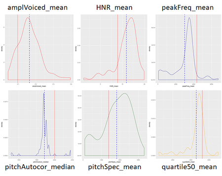
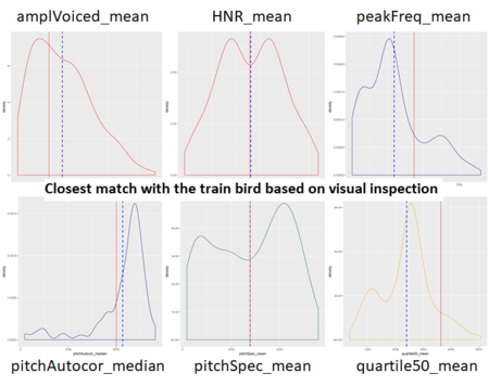
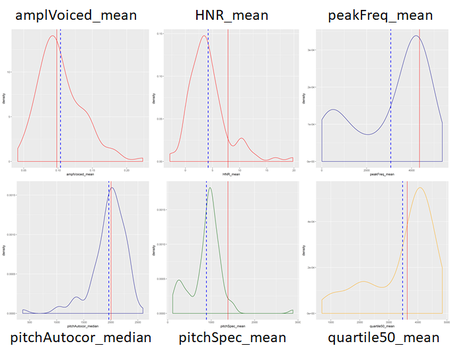
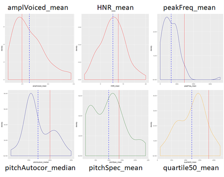
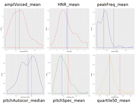
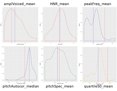
The 6 features of the test files were individually compared with the 6 features of 19 species using density plot in R.
The resultant plots are displayed here for a sample bird for illustration -> Test Sample 3
| Bent-beak Riffraff | Blue-collared Zipper |
| Bombadil | Broad-winged Jojo |
| Canadian Cootamum | Carries Champagne Pipit |
| Darkwing Sparrow | Eastern Corn Skeet |
| Green-tipped Scarlet Pipit | Lesser Birchbeere |
| Orange Pine Plover | Ordinary Snape |
| Pinkfinch | Purple Tooting Tout |
| Qax | Queenscoat |
| Rose-crested Blue Pipit | Scrawny Jay |
| Vermillion Trillian |
Upon visual examination and comparison of the plots, the estimated outcome is:
Note that, both the outcomes do not match as they are based on only visual inspection. Although, by using the second approach, an attempt is made to classify the birds based on the statistical distributions of the species, it is still uncertain to an extent.
Plot for the test birds using the results from distribution analysis:

