ISSS608 2016-17 T3 Assign ANGAD SRIVASTAVA DataPrep
|
|
|
|
|
|
The visualization exercises covered in the next 2 tabs make use of 4 distinct datasets. A brief overview of the data preparation and univariate analysis for all 4 datasets is covered in subsequent sections. These datasets and corresponding analysis has been prepared using both JMP Pro 13 and Tableau.
A brief description of all 4 datasets and preparatory steps is given below:
Geolocation Data
This dataset was created based on the location X and Y coordinate points provided as part of the challenge description. The VAST challenge documentation provides geographical coordinates for all 4 factories and 9 sensors. In addition, a “Type” column was added to differentiate between the type of infrastructural construction (Factory or Sensor) represented by the corresponding coordinates.
Based on the given information, the table below with 4 columns was created which when plotted in a 200x200 coordinate block map shows the following geographical layout of all factories and sensors.
Sensor Data
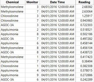
This dataset provided by the VAST challenge documentation in its original format, contains hourly readings for each of the 4 chemicals captured by every Sensor. The number of records span across 3 months i.e. April, August and December, 2016. The adjacent image shows a sample of the dataset provided. Using JMP Pro 13, missing values for this dataset were checked to confirm that all 79,243 rows in this dataset did not have any missing values.
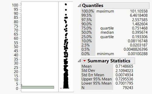
Univariate analysis of the readings also show that the measure of chemical readings is highly skewed. It is noteworthy to highlight the degree of skewness by stating that the 99.5th percentile measure is 6.46 and the maximum value at 101.1. The median reading is at 0.39. These insights have been used in the preparation of selected visualizations, as covered in the next tab.
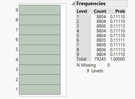
The distribution of the numeric nominal Monitor field was also analysed to ascertain the frequency of all readings for all Sensors. As shown in the adjacent image, all 9 Sensors capture similar number of readings in the 3 months of data provided with minor differences as shown in the frequency count below:
Meteorological Data
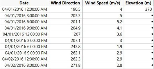
This dataset, as provided by the VAST challenge documentation in its original format, contains atmospheric wind related information. The data covers meteorological readings once every 3 hours with the general wind direction and wind speed captured for that time frame. A snippet of this dataset is shown in the adjacent image.
The relevance of the data field for “Elevation” given in this dataset is unclear and requires additional information. For the purpose of this investigation, this field has been ignored until further information can be provided.
Possible missing values were checked with the following results:
As shown above, there are 2 anomalous records. Further investigations showed that the 2 records are - a empty row and missing values on 30th August, 2016 at 3AM. These 2 records were removed as part of the data cleaning process.
Univariate analysis on the Wind Speed (m/s) shows the frequency of wind speed is well distributed between 0.1 m/s and 6.8 m/s.
Frequency analysis of Wind Direction shows that the wind direction is more skewed between 150 to 360 degrees. Since the given wind direction data is north-facing, the frequency distribution shows that the wind direction is mostly from west to east.
Factory Identification Data
This is a manually created and derived dataset that uses the all of the aforementioned data tables. The purpose and usage of this dataset is to map the chemical readings captured by Sensors at each time frame, with the general wind speed and direction, in an effort to perform geolocation analysis and estimate the factory origin of chemical emissions.
This dataset combines the Sensor data, Meteorological data and Geolocation data to perform an overall geographical analysis. Steps to recreate this dataset are as follows:
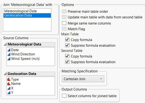
- Using JMP Pro 13, a Cartesian join was performed on Meteorological data and Geolocation data.
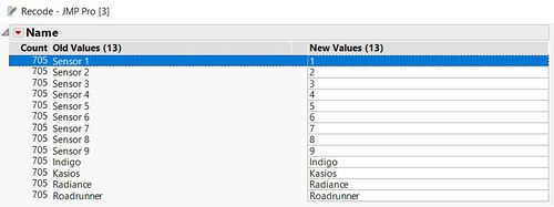
- The Sensor names were recoded to its numerical equivalent before creating a subset, as shown below:
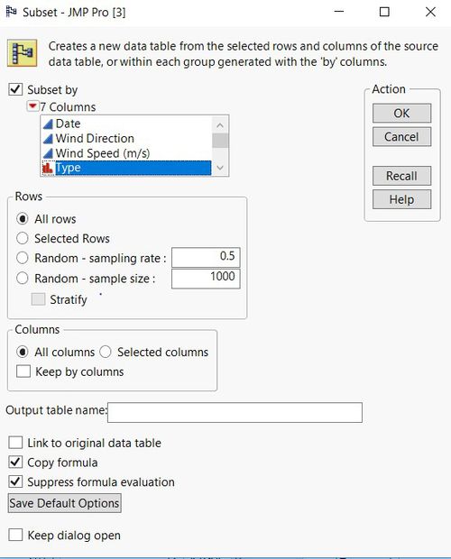
- A subset of this dataset was created to filter out records only for the 9 Sensors and not the 4 factories. This was done using the Subset functionality of JMP on the field “Type”.
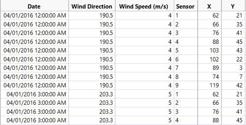
- The resultant Subset created for Sensors with 6,345 rows is shown below:
- Further investigations showed that in order to plot the influence area of each Sensor to trace back to the Factory origin of chemical emissions, any visualization will require a polygonal mapping of its geographically cover the meteorological influence.
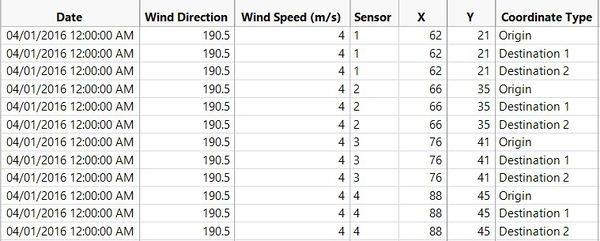
- A Cartesian join was performed on these 2 data tables, which resulted in a consolidated data table with 19,035 records in the following format:
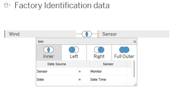
- Finally, this dataset was loaded in Tableau to perform visual analysis. The corresponding Sensor readings for the time frames captured in this dataset were mapped by performing an inner join with the Sensor data in Tableau. The screenshot below shows the inner join performed on Sensor and the Date time fields.
The limitation of the last step is that the analysis performed in Question 3 of Mini Challenge 2 from the VAST Challenge 2017, is based on Sensor readings every 3 hours and not every hour.


