ISSS608 2016-17 T3 Assign CHEN YINJUE Data Analytics
|
|
|
|
|
|
Data Visualization & Insights
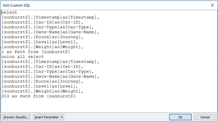
After data preparation, now it's time to draw sunburst chart in tableau. Firstly, open tableau, under ‘Connect’ click ‘Excel’ and then select the Excel file we prepared before. Noted that we should choose ‘open with legacy connection’ in this step so that custom SQL can be used later. Secondly, drag ‘New Custom SQL’ to the area with ‘Drag tables here’ and apply SQL code as below:
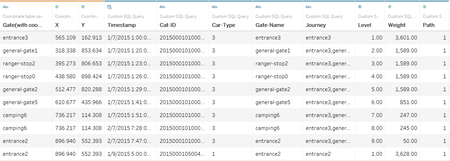
Besides, to lay out the path on the map later, the coordinate table should also be loaded into tableau. So, at the left pane of ‘Data source’, click ‘Add’ (to the right of ‘Connection’) and choose file ‘Coordinate table’. After that, we can select ‘Coordinate table’ under ‘Connection’ and drag ‘Coordinate table.csv’ to join with ‘Custom SQL Query’ by matching the ‘gate name’ of these two sheets. Below shows a sample of output:
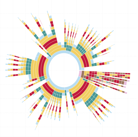
Below is the sunburst diagram showing from level 1 to level 20. To make the graph readable, I purposely colored same gate type with same color:
• Entrance: Blue
• General-Gate: Yellow
• Gate: Brown
• Camp Site: Green
• Ranger-stop: Red
• Ranger-base: Purple
Now, from this sunburst chart, we can summarize several general route patterns:
1. Cars that start from entrance:
• Cars that enter by an entrance and then directly exit the park by an entrance (can be either the same entrance or another entrance):
Entrance > Entrance
• Cars that enter the park and go through one or several general-gate(s) and then exit the park:
Entrance > General-gate(s) > Entrance
• Cars that enter the park for camping (basically includes all routes with camp sites in):
Entrance > … > Camping(s) > … > Entrance
• Cars that enter the park and pass by ranger-stop(s) without going to any camp site:
Entrance > … > Ranger-stop(s) > … > Entrance
• Cars that enter the park and illegally pass by gate(s):
Entrance > … > Gate(s) > … > Entrance
2. Cars that start from ranger-base, which basically should be cars with type ‘2P’. We should pay attention to checking whether there is any other car-type that illegally has this kind of route pattern.
After grabbing an overview as above, next we can begin to divide our datasets… (steps description to be continued)
Briefly, the restructured dataset can be divided into:
• Single path & Single day
• Single path & Multiple days
• Multiple paths
As mentioned before, we have several patterns that can be viewed in sunburst chart already. Therefore, we can further divide the dataset based on route patterns. After that the weight of routes can be calculated and sorted and we pick up records whose routes have relatively bigger weights then others to treat them as major path pattern. Next, we can extract specific data with bigger weights to build calendar view to show the duration (which months or what hours) have heavier traffic for specific path patterns, respectively. Besides, map can be used to demo the corridors. Details of steps are as below:
• Using the general route patterns summarized from sunburst to apply filter on the dataset, which are ‘Single path & Single day’, ‘Single path & Multiple days’ so that the original dataset can be further divided into several worksheets based on routes pattern, name the worksheets respectively (Noted that when using filter, we can just pick out the entire paths of similar route pattern to get a car-id list, then join the whole dataset (without filtering) with the car-id list table).
• Next, each worksheet can be loaded into JMP to calculate weights of different routes (noted only entire paths’ weight will be used to analyse) so that those entire paths with higher number of records can be picked out as major trip patterns.
• Then data will be further extracted from the filtering dataset based on the major trip patterns that we got from step two. By now, the timestamp of these data can be used to build the calendar view so that we can know which duration (months within a year or hours within a day) have bigger traffic volumes.
• Using map to lay out the specific path pattern.
Let’s begin with ‘Single path & Single day’. Based on the analysis steps described above, we can get these several route patterns from the dataset:
• Entrance > Entrance
• Entrance > General-gate(s) > Entrance
• Entrance > … > Camping(s) > … > Entrance
• Entrance > … > Ranger-stop(s) > … > Entrance
For this pattern, there are two paths have highest weights (413 records each path) compared to other routes of similar pattern:
• entrance1 > general-gate7 > general-gate4 > general-gate1 > ranger-stop2 > ranger-stop0 > general-gate2 > entrance2
• entrance2 > general-gate2 > ranger-stop0 > ranger-stop2 > general-gate1 > entrance0


