Mandi Assignment Analysis Procedure
Contents
Question 1: Lake Location
As there is no sensor artifacts in the image which is taken on 2016-09-06, I take this image to locate the position of Boonsong Lake.
First, let's find out where are the waterbody in the image then we can narrow the search area.
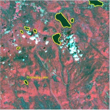
Map B4, B3, B2 to RGB in QGIS to generate the "false-color" image.
In this band combination, water is black. Hence, we can identify the main waterbody which have been highlighted with the yellow line in the preserve area as below.


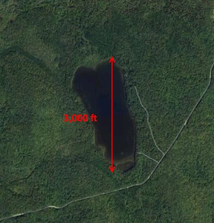
Then we zoom in the image in QGIS and compare the shape of these water area with the image of Boonsong Lake. The water area appears in the left bottom corner should be the Boonsong Lake as their shape are the same. The orientation of the supplied satellite image is also the same with the image of Boonsong Lake, which is oriented north-south.
Next, let's calculate the scale of the supplied satellite image.
I load the reedited "image09_2016_03_06.csv" into Tableau, drag X from the Measure Pane into Columns, Y from Measure Pane into Rows. Choose the Measure method as "Dimension".
As there are 651 rows and columns, I fix the range of x axis and y axis from 0 to 650.
X=0, Y=0 refers to the pixel in the upper left corner of the image. Similarly, the bottom right pixel of the image is X=650, Y=650.
To map the pixel in the dashboard with the real image, I reversed the scale of Y axis.
Drag the NDVI from the Measure Pane to dashboard area and set the measure method of NDVI as "Dimension" in the Marks Card.
Choose "Square" from the drop-down list and set the size as the smallest. Then it will be easier to locate the Boonsong Lake as each square will represent one pixel.
Now we still cannot recognize the preserve area in the map. Drag NDVI to the Color card then different regions in the area will be shown in different colors.
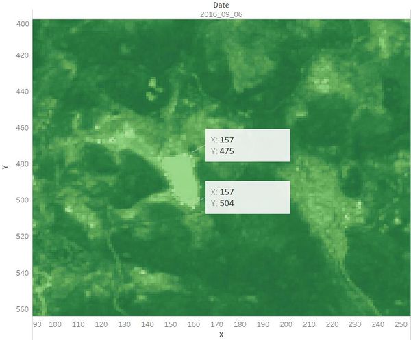
We can see that the Boonsong Lake is at the left bottom corner of the dashboard.
Use the view toolbar to zoom in the dashboard and add annotation to show the X, Y coordinates at the top pixel and bottom pixel of the Boonsong Lake respectively.
Hence, the length of a pixel is 3000/(504 - 475+1) ft, equals to 100 ft. Then the area of one pixel is 100 * 100 = 10000 square ft.
As the satellite image has 651*651 pixels, the actual scale of the region is 651*651*10000 square ft = 4,238,010,000 square ft.
