Difference between revisions of "ISSS608 2016-17 T3 Group5 Immigration Methodology"
Xqchen.2016 (talk | contribs) |
|||
| (18 intermediate revisions by 2 users not shown) | |||
| Line 9: | Line 9: | ||
[[ISSS608_2016-17_T3_Assign__Group5_Immigration_Proposal| <font color="#FFFFFF">Proposal</font>]] | [[ISSS608_2016-17_T3_Assign__Group5_Immigration_Proposal| <font color="#FFFFFF">Proposal</font>]] | ||
| − | | style="font-family:Century Gothic; font-size:100%; solid #1B338F; background:#2B3856; text-align:center;" width=" | + | | style="font-family:Century Gothic; font-size:100%; solid #1B338F; background:#2B3856; text-align:center;" width="16.6%" | |
; | ; | ||
[[ISSS608_2016-17_T3_Group5_Immigration_Intro| <font color="#FFFFFF">Introduction</font>]] | [[ISSS608_2016-17_T3_Group5_Immigration_Intro| <font color="#FFFFFF">Introduction</font>]] | ||
| − | | style="font-family:Century Gothic; font-size:100%; solid #1B338F; background:#2B3856; text-align:center;" width=" | + | | style="font-family:Century Gothic; font-size:100%; solid #1B338F; background:#2B3856; text-align:center;" width="16.6%" | |
; | ; | ||
[[ISSS608_2016-17_T3_Group5_Immigration_Methodology| <font color="#FFFFFF">Methodology</font>]] | [[ISSS608_2016-17_T3_Group5_Immigration_Methodology| <font color="#FFFFFF">Methodology</font>]] | ||
| − | | style="font-family:Century Gothic; font-size:100%; solid #1B338F; background:#2B3856; text-align:center;" width=" | + | | style="font-family:Century Gothic; font-size:100%; solid #1B338F; background:#2B3856; text-align:center;" width="16.6%" | |
; | ; | ||
[[ISSS608_2016-17_T3_Group5_Immigration_Application| <font color="#FFFFFF">Application</font>]] | [[ISSS608_2016-17_T3_Group5_Immigration_Application| <font color="#FFFFFF">Application</font>]] | ||
| − | | style="font-family:Century Gothic; font-size:100%; solid #1B338F; background:#2B3856; text-align:center;" width=" | + | | style="font-family:Century Gothic; font-size:100%; solid #1B338F; background:#2B3856; text-align:center;" width="16.6%" | |
; | ; | ||
[[ISSS608_2016-17_T3_Assign__Group5_Immigration_Poster| <font color="#FFFFFF">Poster</font>]] | [[ISSS608_2016-17_T3_Assign__Group5_Immigration_Poster| <font color="#FFFFFF">Poster</font>]] | ||
| − | | style="font-family:Century Gothic; font-size:100%; solid #1B338F; background:#2B3856; text-align:center;" width=" | + | | style="font-family:Century Gothic; font-size:100%; solid #1B338F; background:#2B3856; text-align:center;" width="16.6%" | |
| − | ; | + | ; |
| + | [[ISSS608_2016-17_T3_Assign__Group5_Immigration_Discussion| <font color="#FFFFFF">Discussion</font>]] | ||
| + | |||
| + | | style="font-family:Century Gothic; font-size:100%; solid #1B338F; background:#2B3856; text-align:center;" width="16.6%" | | ||
| + | ; | ||
|} | |} | ||
| − | ==Design Framework | + | ==Design Framework: Addressing the analytic gap== |
| − | |||
| − | |||
Currently, we observe that attempts at visualising migration flows tend to be more descriptive than analytic, choosing to focus on the presentation of the directions and the volumes of the migration flows rather than providing any analytical link explaining the flows. This tendency seems to partially stem from the complexity of the phenomenon of migration, which makes explaining its flows from a general level difficult. Ernest Ravenstein - the grandfather of migration theory - theorised migration as being caused by push-pull factors; where “push” factors in the origin country propel people to emigrate and “pull” factors attract people to immigrate. Most contemporary approaches to migration – be it neoclassical economics, segmented labour market theory, or the world systems approach – have fundamentally not departed from Ravenstein’s thesis. However, as the reasons that people migrate become more varied, a more comprehensive theory of migration becomes difficult to formulate. Hence, most studies of migration that move beyond a descriptive level tend to address the effects and implications of migration rather than the causes of migration itself. However, as scholars and policy makers focused on more context-focused approaches and “middle-level” theoretical explanations to the study of migration, they tend to lose sight of how variables at the more structural level - such as macro-economic indicators, political regime, sociocultural factors and other country level attributes - could actually play a part in influencing migration patterns. | Currently, we observe that attempts at visualising migration flows tend to be more descriptive than analytic, choosing to focus on the presentation of the directions and the volumes of the migration flows rather than providing any analytical link explaining the flows. This tendency seems to partially stem from the complexity of the phenomenon of migration, which makes explaining its flows from a general level difficult. Ernest Ravenstein - the grandfather of migration theory - theorised migration as being caused by push-pull factors; where “push” factors in the origin country propel people to emigrate and “pull” factors attract people to immigrate. Most contemporary approaches to migration – be it neoclassical economics, segmented labour market theory, or the world systems approach – have fundamentally not departed from Ravenstein’s thesis. However, as the reasons that people migrate become more varied, a more comprehensive theory of migration becomes difficult to formulate. Hence, most studies of migration that move beyond a descriptive level tend to address the effects and implications of migration rather than the causes of migration itself. However, as scholars and policy makers focused on more context-focused approaches and “middle-level” theoretical explanations to the study of migration, they tend to lose sight of how variables at the more structural level - such as macro-economic indicators, political regime, sociocultural factors and other country level attributes - could actually play a part in influencing migration patterns. | ||
| Line 39: | Line 41: | ||
==Data Description== | ==Data Description== | ||
| − | <big>Migration data ( | + | <big>Migration data (Global Migration Info)</big> |
| − | |||
| − | |||
| − | |||
| − | |||
| − | |||
| + | The bilateral migration data used was from [http://www.global-migration.info/ Global Migration Info] which contains data on bilateral flows between 196 countries that are estimated from sequential stock tables. These data are comparable across countries and capture the number of people who changed their country of residence over 4 five-year periods): 1990-1995, 1995-2000, 2000-2005, 2005-2010. The estimates however, reflect migration transitions and thus cannot be compared to annual movements flow data published by United Nations and Eurostat. | ||
<big>Polity data (Polity IV dataset)</big> | <big>Polity data (Polity IV dataset)</big> | ||
| − | The Polity IV dataset covers all major, independent states in the global system over the period 1800-2015 (i.e., states with a total population of 500,000 or more in the most recent year | + | The [http://www.systemicpeace.org/inscr/p4v2015.xls Polity IV dataset] contains data on authority characteristics of states in the world system for purposes of comparative, quantitative analysis of political regimes and is widely used in political science research. Its conceptual scheme examines the qualities of democratic and autocratic authority in government institutions, and is used in our project to help construct the political dimension of the country attribute profile. This dataset covers all major, independent states in the global system over the period 1800-2015 (i.e., states with a total population of 500,000 or more in the most recent year. Currently, the dataset contains 167 countries. |
| − | |||
| − | |||
| − | |||
| − | + | <big>Economic Data (World Development Indicators)</big> | |
| + | For the economic dimension of our country profiles, we are drawing data from [http://data.worldbank.org/data-catalog/world-development-indicators World Bank's World Development Indicators]. | ||
| + | The world development indicators show the different attributes of different countries starts from 1985 to 2010. We are including 69 quantitative attributes such as GDP, fertility, CO2, inflation, health expense, unemployment and so on. These factors were selected based on two main considerations: whether they were general enough to apply to all countries and whether there were sufficient data points within them for most ccountries. The full list of initial WDI variables are listed below. Do note that some of these variables were eventually dropped in the data joining process due to too many NA values. | ||
| + | "electricity%", #Access to electricity (% of population) | ||
| + | "ado.fertility", #Adolescent fertility rate (births per 1,000 women ages 15-19) | ||
| + | "agri.land", #Agricultural land (sq. km) | ||
| + | "arable.land%", #Arable land (% of land area) | ||
| + | "personnel", #Armed forces personnel, total | ||
| + | "birth.rate", #Birth rate, crude (per 1,000 people) | ||
| + | "CO2", # CO2 emissions (kt) | ||
| + | "death.rate", #Death rate, crude (per 1,000 people) | ||
| + | "energy.import", #Energy imports, net (% of energy use) | ||
| + | "fertility", #Fertility rate, total (births per woman) | ||
| + | "food.export", #Food exports (% of merchandise exports) | ||
| + | "food.import", #TM.VAL.FOOD.ZS.UN | ||
| + | "FDI", #Foreign direct investment, net (BoP, current US$) | ||
| + | "FDI.inflows", #Foreign direct investment, net inflows (BoP, current US$) | ||
| + | "forest", #Forest area (sq. km) | ||
| + | "GDP", #GDP (current US$) | ||
| + | "growth", #GDP growth (annual %) | ||
| + | "GDPpc", #GDP per capita (current US$) | ||
| + | "GDPpc.growth", #GDP per capita growth (annual %) | ||
| + | "gini", #GINI index | ||
| + | "gov.expen", #General government final consumption expenditure (current US$) | ||
| + | "savings", #Gross domestic savings (% of GDP) | ||
| + | "health.expen", #Health expenditure, public (% of GDP) | ||
| + | "health.expenpc", #Health expenditure per capita (current US$) | ||
| + | "inflation", #Inflation, GDP deflator (annual %) | ||
| + | "tourism.arrival", #International tourism, number of arrivals | ||
| + | "tourism.depart", #International tourism, number of departures | ||
| + | "labor.f", # Labor force participation rate, female (% of female population ages 15-24) | ||
| + | "labor.m", # Labor force participation rate, male (% of male population ages 15-24) | ||
| + | "labor.rate", #Labor force participation rate, total (% of total population ages 15-24) | ||
| + | "m:f.labor.rate", # Ratio of female to male labor force participation rate (%) | ||
| + | "labor",# Labor force, total | ||
| + | "land",# Land area (sq. km) | ||
| + | "life.f", # Life expectancy at birth, female (years) | ||
| + | "life", # Life expectancy at birth, total (years) | ||
| + | "life.m", # Life expectancy at birth, male (years) | ||
| + | "literacy", # Literacy rate, adult total (% of people ages 15 and above) | ||
| + | "mortality.f", # Mortality rate, adult, female (per 1,000 female adults) | ||
| + | "mortality.m", # Mortality rate, adult, male (per 1,000 male adults) | ||
| + | "aid.bilateral", # Net bilateral aid flows from DAC donors, Total (current US$) | ||
| + | "aid.US", # Net bilateral aid flows from DAC donors, United States (current US$) | ||
| + | "migration", # Net migration | ||
| + | "aid", # Net official aid received (current US$) | ||
| + | "oil", # Oil rents (% of GDP) | ||
| + | "pop.y", # Population ages 0-14 (% of total) | ||
| + | "pop.m", # Population ages 15-64 (% of total) | ||
| + | "pop.s", # Population ages 65 and above (% of total) | ||
| + | "pop", # Population, total | ||
| + | "age.dep", # Age dependency ratio (% of working-age population) | ||
| + | "age.dep.s", # Age dependency ratio, old (% of working-age population) | ||
| + | "age.dep.y", # Age dependency ratio, young (% of working-age population) | ||
| + | "pop.density", # Population density (people per sq. km of land area) | ||
| + | "pop.growth", # Population growth (annual %) | ||
| + | "pop.f", # Population, female (% of total) | ||
| + | "HIV", # Prevalence of HIV, total (% of population ages 15-49) | ||
| + | "railway", # Railways, passengers carried (million passenger-km) | ||
| + | "rural", # Rural population (% of total population) | ||
| + | "urbanization", # Urban population (% of total) | ||
| + | "urban.pop", # Urban population | ||
| + | "urban.pop.g", # Urban population growth (annual %) | ||
| + | "pri.edu", # School enrollment, primary (% gross) | ||
| + | "sec.edu", # School enrollment, secondary (% gross) | ||
| + | "tariff", # Tariff rate, applied, simple mean, all products (%) | ||
| + | "telephone", # Telephone lines (per 100 people) | ||
| + | "resources", # Total natural resources rents (% of GDP) | ||
| + | "trade%", #Trade (% of GDP) | ||
| + | "unemployment.f", # Unemployment, female (% of female labor force) | ||
| + | "unemployment.m", # Unemployment, male (% of male labor force) | ||
| + | "unemployment", # Unemployment, total (% of total labor force) | ||
| − | <big>Hofstede's cultural dimensions data</big> | + | <big> Sociocultural data (Hofstede's cultural dimensions data)</big> |
| − | Hofstede cultural dimensions conceptualises national cultural as comprising of 6 dimensions: the Power Distance Index (PDI), Individualism versus Collectivism (IDV), Masculinity versus Femininity (MAS), Uncertainty Avoidance Index (UAI), Long Term Orientation versus Short Term Normative Orientation (LTO) and Indulgence versus Restraint (IND). [[file: Culture.png|border|thumb|500px]] | + | Finally, to construct the socioeconomic profile of our countries, we turn to [http://www.geerthofstede.nl/ Geert Hofstede's international study] on the 6 cultural dimensions of countries. Hofstede's cultural dimensions conceptualises national cultural as comprising of 6 dimensions: the Power Distance Index (PDI), Individualism versus Collectivism (IDV), Masculinity versus Femininity (MAS), Uncertainty Avoidance Index (UAI), Long Term Orientation versus Short Term Normative Orientation (LTO) and Indulgence versus Restraint (IND). [[file: Culture.png|border|thumb|500px]] |
*PDI score measures the degree to which les powerful members of society accept the unequal way in which power is distributed. A country with high PDI score suggests that power differences are accepted as the norm while a low PDI score suggests that people have more focus on social justice issues and strive to equalise how power is distributed. | *PDI score measures the degree to which les powerful members of society accept the unequal way in which power is distributed. A country with high PDI score suggests that power differences are accepted as the norm while a low PDI score suggests that people have more focus on social justice issues and strive to equalise how power is distributed. | ||
| Line 74: | Line 140: | ||
The data collected for Hofstede’s Cultural Dimensions dataset (https://geert-hofstede.com/national-culture.html) originate from different periods. The first scores from more than 70 countries – of which only 40 were used – were collated between 1967 and 1973. Later editions expanded the range of countries and the current third edition covers a total of 111 countries. However, Hofstede argues that as “culture changes very slowly, the scores can be considered up to date”. | The data collected for Hofstede’s Cultural Dimensions dataset (https://geert-hofstede.com/national-culture.html) originate from different periods. The first scores from more than 70 countries – of which only 40 were used – were collated between 1967 and 1973. Later editions expanded the range of countries and the current third edition covers a total of 111 countries. However, Hofstede argues that as “culture changes very slowly, the scores can be considered up to date”. | ||
| + | |||
| + | ==Design Principles== | ||
| + | |||
| + | Having distilled several design principles through the review of past visualisations of migration, our design was driven by these considerations: | ||
| + | |||
| + | *For Data Visualisation: | ||
| + | |||
| + | # We needed a way to successfully represent all the migration flows between source and destination countries | ||
| + | # We needed a way to compare between the attributes of source and destination countries | ||
| + | # We needed a way to allow users to compare between the 5-yearly migration dataset and the annual data of the country attributes. | ||
| + | |||
| + | *For User Interface Design: | ||
| + | |||
| + | # To allow the user to creatively explore, within a sandbox environment, the relationships between country attributes and the migration flows. | ||
| + | # To embed controls within the user interface that will allow user to explore without being overwhelmed by too many country-pairs or attributes | ||
| + | # To provide some form of prior analysis or recommendation system to reduce the problem of multidimensionality of the country attributes and allow users to get a better sense of how to choose which attributes to study. | ||
| + | |||
| + | |||
| + | We developed an analytical framework to explore determinants of migration i.e. how the attributes of source and destination countries are related to in and out migration rates of these countries. We decided to build our data visualisation dashboard using Rstudio and R shiny as R is a flexible and powerful language that is good at data manipulation and has many packages for data visualisation. Using R/Shiny and other packages, we attempted to integrate bilateral migration flow data with data describing the characteristics of both source and destination countries, drawing data from the World Bank, the Polity IV dataset, and measures from the Hofstede’s Cultural Dimension Theory. This culminated in the design of an analytical dashboard that allows users to perform exploratory data analysis to aid policy and academic research on migration. | ||
| + | |||
| + | |||
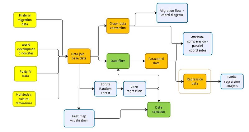
| + | Given its utility as observed in our review of past work, we decided to represent the migration flows using a chord diagram, and represent the country attributes using a parallel coordinate plot. We also wanted to create an automated variable selection function that recommends to the user which variables are the most important so that the user does not need to shuffle through more than a hundred attributes before finding the one of interest. We also decided to provide a series of controls for the user to select and choose the origin and destination countries through specifying their respective regions. That way, when the user explores, he or she can better manage what countries are represented. At the same time, the partial loading of the dataset will reduce processing overheads, especially on slower computers. We also wanted users to be able to toggle between different time periods for both migration flows as well as country attributes so that they can better explore and compare whether different time periods of the attributes had any relation with the migration flows. Finally, we wanted to provide a partial regression analysis function so that the user can understand, based on what attributes were selected, the effect in which the attribute(s) in question had on the migration flows. The process flow of our app is presented below: | ||
| + | |||
| + | [[file:Process.jpeg|800px]] | ||
Latest revision as of 23:22, 6 August 2017
 Group 5 - Why Did the Migrant Cross the Road?
|
|
|
|
|
|
|
|
Design Framework: Addressing the analytic gap
Currently, we observe that attempts at visualising migration flows tend to be more descriptive than analytic, choosing to focus on the presentation of the directions and the volumes of the migration flows rather than providing any analytical link explaining the flows. This tendency seems to partially stem from the complexity of the phenomenon of migration, which makes explaining its flows from a general level difficult. Ernest Ravenstein - the grandfather of migration theory - theorised migration as being caused by push-pull factors; where “push” factors in the origin country propel people to emigrate and “pull” factors attract people to immigrate. Most contemporary approaches to migration – be it neoclassical economics, segmented labour market theory, or the world systems approach – have fundamentally not departed from Ravenstein’s thesis. However, as the reasons that people migrate become more varied, a more comprehensive theory of migration becomes difficult to formulate. Hence, most studies of migration that move beyond a descriptive level tend to address the effects and implications of migration rather than the causes of migration itself. However, as scholars and policy makers focused on more context-focused approaches and “middle-level” theoretical explanations to the study of migration, they tend to lose sight of how variables at the more structural level - such as macro-economic indicators, political regime, sociocultural factors and other country level attributes - could actually play a part in influencing migration patterns.
Our ISSS608 project would like to address this gap, moving beyond the current visualisations and attempt to create a dashboard application that could provide an additional analytic lens. We fall back to Ravenstein’s theory of migration, by looking at how country attributes influence migration flows. In order to provide a more holistic overview, we decide to combine economic data from the World Bank, data on political regime characteristics from the Polity IV database, and sociocultural measures from Geert Hofstede’s 6 Cultural Dimensions to provide create a general profile for countries. To study migration flows, we decided upon the World Bank Global Bilateral Migration dataset. This dashboard application focuses on allowing the user to explore not only the migration flows, but the push and pull factors behind these flows as well by visualizing the various country attributes as differential levels that may correlate with the magnitude and degree of migration.
Data Description
Migration data (Global Migration Info)
The bilateral migration data used was from Global Migration Info which contains data on bilateral flows between 196 countries that are estimated from sequential stock tables. These data are comparable across countries and capture the number of people who changed their country of residence over 4 five-year periods): 1990-1995, 1995-2000, 2000-2005, 2005-2010. The estimates however, reflect migration transitions and thus cannot be compared to annual movements flow data published by United Nations and Eurostat.
Polity data (Polity IV dataset)
The Polity IV dataset contains data on authority characteristics of states in the world system for purposes of comparative, quantitative analysis of political regimes and is widely used in political science research. Its conceptual scheme examines the qualities of democratic and autocratic authority in government institutions, and is used in our project to help construct the political dimension of the country attribute profile. This dataset covers all major, independent states in the global system over the period 1800-2015 (i.e., states with a total population of 500,000 or more in the most recent year. Currently, the dataset contains 167 countries.
Economic Data (World Development Indicators)
For the economic dimension of our country profiles, we are drawing data from World Bank's World Development Indicators. The world development indicators show the different attributes of different countries starts from 1985 to 2010. We are including 69 quantitative attributes such as GDP, fertility, CO2, inflation, health expense, unemployment and so on. These factors were selected based on two main considerations: whether they were general enough to apply to all countries and whether there were sufficient data points within them for most ccountries. The full list of initial WDI variables are listed below. Do note that some of these variables were eventually dropped in the data joining process due to too many NA values.
 "electricity%", #Access to electricity (% of population)
 "ado.fertility",  #Adolescent fertility rate (births per 1,000 women ages 15-19)
 "agri.land", #Agricultural land (sq. km)
 "arable.land%", #Arable land (% of land area)
 "personnel", #Armed forces personnel, total
 "birth.rate", #Birth rate, crude (per 1,000 people)
 "CO2", #	CO2 emissions (kt)
 "death.rate", #Death rate, crude (per 1,000 people)
 "energy.import", #Energy imports, net (% of energy use)
 "fertility", #Fertility rate, total (births per woman)
 "food.export", #Food exports (% of merchandise exports)
 "food.import", #TM.VAL.FOOD.ZS.UN
 "FDI", #Foreign direct investment, net (BoP, current US$)
 "FDI.inflows", #Foreign direct investment, net inflows (BoP, current US$)
 "forest", #Forest area (sq. km)
 "GDP", #GDP (current US$)
 "growth", #GDP growth (annual %)
 "GDPpc", #GDP per capita (current US$)
 "GDPpc.growth", #GDP per capita growth (annual %)
 "gini", #GINI index
 "gov.expen", #General government final consumption expenditure (current US$)
 "savings", #Gross domestic savings (% of GDP)
 "health.expen", #Health expenditure, public (% of GDP)
 "health.expenpc", #Health expenditure per capita (current US$)
 "inflation", #Inflation, GDP deflator (annual %)
 "tourism.arrival", #International tourism, number of arrivals
 "tourism.depart",	#International tourism, number of departures
 "labor.f", #	Labor force participation rate, female (% of female population ages 15-24)
 "labor.m", #	Labor force participation rate, male (% of male population ages 15-24)
 "labor.rate", #Labor force participation rate, total (% of total population ages 15-24)
 "m:f.labor.rate", #	Ratio of female to male labor force participation rate (%)
 "labor",#	Labor force, total
 "land",#	Land area (sq. km)
 "life.f",  #	Life expectancy at birth, female (years)
 "life",  #	Life expectancy at birth, total (years)
 "life.m",  #	Life expectancy at birth, male (years)
 "literacy",  #	Literacy rate, adult total (% of people ages 15 and above)
 "mortality.f",  #	Mortality rate, adult, female (per 1,000 female adults)
 "mortality.m",  #	Mortality rate, adult, male (per 1,000 male adults)
 "aid.bilateral",  #	Net bilateral aid flows from DAC donors, Total (current US$)
 "aid.US",  #	Net bilateral aid flows from DAC donors, United States (current US$)
 "migration",  #			Net migration
 "aid",  #	Net official aid received (current US$)
 "oil",  #	 Oil rents (% of GDP)
 "pop.y",  #	Population ages 0-14 (% of total)
 "pop.m",  #	Population ages 15-64 (% of total)
 "pop.s",  #	Population ages 65 and above (% of total)
 "pop",  #			Population, total
 "age.dep",  #	Age dependency ratio (% of working-age population)
 "age.dep.s",  #	Age dependency ratio, old (% of working-age population)
 "age.dep.y",  #	Age dependency ratio, young (% of working-age population)
 "pop.density",  #	Population density (people per sq. km of land area)
 "pop.growth",  #	Population growth (annual %)
 "pop.f",  #	Population, female (% of total)
 "HIV",  #	Prevalence of HIV, total (% of population ages 15-49)
 "railway",  #		Railways, passengers carried (million passenger-km)
 "rural",  #	Rural population (% of total population)
 "urbanization",  #	Urban population (% of total)
 "urban.pop",  #	Urban population
 "urban.pop.g",  #	Urban population growth (annual %)
 "pri.edu",  #	School enrollment, primary (% gross)
 "sec.edu",  #	School enrollment, secondary (% gross)
 "tariff",  #	Tariff rate, applied, simple mean, all products (%)
 "telephone",  #	Telephone lines (per 100 people)
 "resources",  #			Total natural resources rents (% of GDP)
 "trade%", #Trade (% of GDP)
 "unemployment.f",  #	Unemployment, female (% of female labor force)
 "unemployment.m",  #	Unemployment, male (% of male labor force)
 "unemployment",  #	Unemployment, total (% of total labor force)
Sociocultural data (Hofstede's cultural dimensions data)
Finally, to construct the socioeconomic profile of our countries, we turn to Geert Hofstede's international study on the 6 cultural dimensions of countries. Hofstede's cultural dimensions conceptualises national cultural as comprising of 6 dimensions: the Power Distance Index (PDI), Individualism versus Collectivism (IDV), Masculinity versus Femininity (MAS), Uncertainty Avoidance Index (UAI), Long Term Orientation versus Short Term Normative Orientation (LTO) and Indulgence versus Restraint (IND).

- PDI score measures the degree to which les powerful members of society accept the unequal way in which power is distributed. A country with high PDI score suggests that power differences are accepted as the norm while a low PDI score suggests that people have more focus on social justice issues and strive to equalise how power is distributed.
- IDV scores measures the permeation of the culture of individualism within societies. A higher IDV score suggests that societal values are more individualistic and self-image is defined by “I” rather than “we”. A low IDV score suggests the opposite, that societies have a more collectivist outlook and practice more communitarian values.
- The MAS dimension represents whether success in society is defined through a culture of “achievement, heroism, assertiveness and material rewards” (high score; “masculine”) or whether it instead prefers “cooperation, modesty, caring for the weak, and quality of life” (low score; “feminine”).
- UAI measures risk aversion and how much countries will feel when faced with uncertainty. When UAI is high, societal values manifest in a low tolerance of unorthodoxy and contestation where strict codes of behaviour are enforced. In low UAI countries, practice and what works counts more, and people are more flexible and relaxed about what the proper way of doing things are.
- LTO is related and somewhat similar to UAI, where it measures how societies deal with their own historicity and manage challenges in the present and the future. Countries with low LTO tend to be more suspicious of societal change and countries with high LTO tend to prefer more pragmatic approaches to dealing with the future.
- IND scores measure how societies deal with basic gratification needs. High IND societies are more predisposed to having fun and enjoying life while low IND societies delay gratification and regulate it through strict social norms and codes.
The data collected for Hofstede’s Cultural Dimensions dataset (https://geert-hofstede.com/national-culture.html) originate from different periods. The first scores from more than 70 countries – of which only 40 were used – were collated between 1967 and 1973. Later editions expanded the range of countries and the current third edition covers a total of 111 countries. However, Hofstede argues that as “culture changes very slowly, the scores can be considered up to date”.
Design Principles
Having distilled several design principles through the review of past visualisations of migration, our design was driven by these considerations:
- For Data Visualisation:
- We needed a way to successfully represent all the migration flows between source and destination countries
- We needed a way to compare between the attributes of source and destination countries
- We needed a way to allow users to compare between the 5-yearly migration dataset and the annual data of the country attributes.
- For User Interface Design:
- To allow the user to creatively explore, within a sandbox environment, the relationships between country attributes and the migration flows.
- To embed controls within the user interface that will allow user to explore without being overwhelmed by too many country-pairs or attributes
- To provide some form of prior analysis or recommendation system to reduce the problem of multidimensionality of the country attributes and allow users to get a better sense of how to choose which attributes to study.
We developed an analytical framework to explore determinants of migration i.e. how the attributes of source and destination countries are related to in and out migration rates of these countries. We decided to build our data visualisation dashboard using Rstudio and R shiny as R is a flexible and powerful language that is good at data manipulation and has many packages for data visualisation. Using R/Shiny and other packages, we attempted to integrate bilateral migration flow data with data describing the characteristics of both source and destination countries, drawing data from the World Bank, the Polity IV dataset, and measures from the Hofstede’s Cultural Dimension Theory. This culminated in the design of an analytical dashboard that allows users to perform exploratory data analysis to aid policy and academic research on migration.
Given its utility as observed in our review of past work, we decided to represent the migration flows using a chord diagram, and represent the country attributes using a parallel coordinate plot. We also wanted to create an automated variable selection function that recommends to the user which variables are the most important so that the user does not need to shuffle through more than a hundred attributes before finding the one of interest. We also decided to provide a series of controls for the user to select and choose the origin and destination countries through specifying their respective regions. That way, when the user explores, he or she can better manage what countries are represented. At the same time, the partial loading of the dataset will reduce processing overheads, especially on slower computers. We also wanted users to be able to toggle between different time periods for both migration flows as well as country attributes so that they can better explore and compare whether different time periods of the attributes had any relation with the migration flows. Finally, we wanted to provide a partial regression analysis function so that the user can understand, based on what attributes were selected, the effect in which the attribute(s) in question had on the migration flows. The process flow of our app is presented below: