Difference between revisions of "Mandi Assignment Data Preparation"
| (2 intermediate revisions by the same user not shown) | |||
| Line 4: | Line 4: | ||
{|style="background-color:#1B338F;" width="100%" cellspacing="0" cellpadding="0" valign="top" border="0" | | {|style="background-color:#1B338F;" width="100%" cellspacing="0" cellpadding="0" valign="top" border="0" | | ||
| − | | style="font-size:100%; solid #000000; background:#2B3856; text-align:center;" width=" | + | | style="font-size:100%; solid #000000; background:#2B3856; text-align:center;" width="16.6%" | |
[[ISSS608_2016-17_T3_Assign_LUO_MANDI| <font color="#FFFFFF">Introduction</font>]] | [[ISSS608_2016-17_T3_Assign_LUO_MANDI| <font color="#FFFFFF">Introduction</font>]] | ||
| − | | style="font-size:100%; solid #1B338F; background:#2B3856; text-align:center;" width=" | + | | style="font-size:100%; solid #1B338F; background:#2B3856; text-align:center;" width="16.6%" | |
[[Mandi_Assignment_Data_Preparation| <font color="#FFFFFF">Data Preparation</font>]] | [[Mandi_Assignment_Data_Preparation| <font color="#FFFFFF">Data Preparation</font>]] | ||
| − | | style="font-size:100%; solid #1B338F; background:#2B3856; text-align:center;" width=" | + | | style="font-size:100%; solid #1B338F; background:#2B3856; text-align:center;" width="16.6%" | |
[[Mandi_Assignment_Analysis_Procedure| <font color="#FFFFFF">Data Exploration</font>]] | [[Mandi_Assignment_Analysis_Procedure| <font color="#FFFFFF">Data Exploration</font>]] | ||
| − | | style="font-size:100%; solid #1B338F; background:#2B3856; text-align:center;" width=" | + | | style="font-size:100%; solid #1B338F; background:#2B3856; text-align:center;" width="16.6%" | |
[[Mandi_Assignment_Final_Answer| <font color="#FFFFFF">Final Answer</font>]] | [[Mandi_Assignment_Final_Answer| <font color="#FFFFFF">Final Answer</font>]] | ||
| − | | style="font-size:100%; solid #1B338F; background:#2B3856; text-align:center;" width=" | + | | style="font-size:100%; solid #1B338F; background:#2B3856; text-align:center;" width="16.6%" | |
| + | [[Mandi_Assignment_Visualization| <font color="#FFFFFF">Visualization Result</font>]] | ||
| + | |||
| + | | style="font-size:100%; solid #1B338F; background:#2B3856; text-align:center;" width="16.6%" | | ||
[[Mandi_Assignment_Comments| <font color="#FFFFFF">Comments</font>]] | [[Mandi_Assignment_Comments| <font color="#FFFFFF">Comments</font>]] | ||
|} | |} | ||
| Line 25: | Line 28: | ||
==Noise Data Filtering== | ==Noise Data Filtering== | ||
There are totally 12 TIF files. I load them into QGIS and mapped B3, B2 and B1 to RGB and generate the "true-color" images as below. <br/> | There are totally 12 TIF files. I load them into QGIS and mapped B3, B2 and B1 to RGB and generate the "true-color" images as below. <br/> | ||
| − | [[File:noise_check.JPG]] | + | [[File:noise_check.JPG|1000px]] |
<br/> | <br/> | ||
When looking at these "true-color" images, there are three images in which the preserve area cannot be seen clearly due to the clouds. <br/> | When looking at these "true-color" images, there are three images in which the preserve area cannot be seen clearly due to the clouds. <br/> | ||
| Line 36: | Line 39: | ||
Compared to others, the image taken on 2016-09-06 is much more clear. It is a good choice to locate the position of the Boonsong Lake in the preserve. <br/> | Compared to others, the image taken on 2016-09-06 is much more clear. It is a good choice to locate the position of the Boonsong Lake in the preserve. <br/> | ||
| − | == | + | ==Load Data into JMP== |
| − | ===Concatenate data=== | + | ===Concatenate Data=== |
| − | + | To compare the changes in different days, I concatenate the data in JMP as below. It will create one column as the "Source Table".<br/> | |
| + | [[File:Concatenate.jpg|500px]] <br/> | ||
| + | ===Add Date=== | ||
| + | Then I add a column "Date", which shows the date of the image. <br/><br/> | ||
| + | [[File:Date.jpg|450px]] | ||
===NVDI Calculation=== | ===NVDI Calculation=== | ||
| + | According to the definition of NDVI (Normalized Difference Vegetation Index): NDVI = (B4 - B3) / (B4 + B3), I add the formula to calculate the NDVI value. <br/> | ||
| + | [[File:NDVIC.jpg|400px]] | ||
==Create Bins in Tableau== | ==Create Bins in Tableau== | ||
Latest revision as of 23:51, 16 July 2017
The data set has two forms of image data: TIF files and ASCII files. Both of them contains same information.
I use QGIS to load the TIF files for visualization and JMP to load the ASCII files for stacking data.
Contents
Noise Data Filtering
There are totally 12 TIF files. I load them into QGIS and mapped B3, B2 and B1 to RGB and generate the "true-color" images as below.
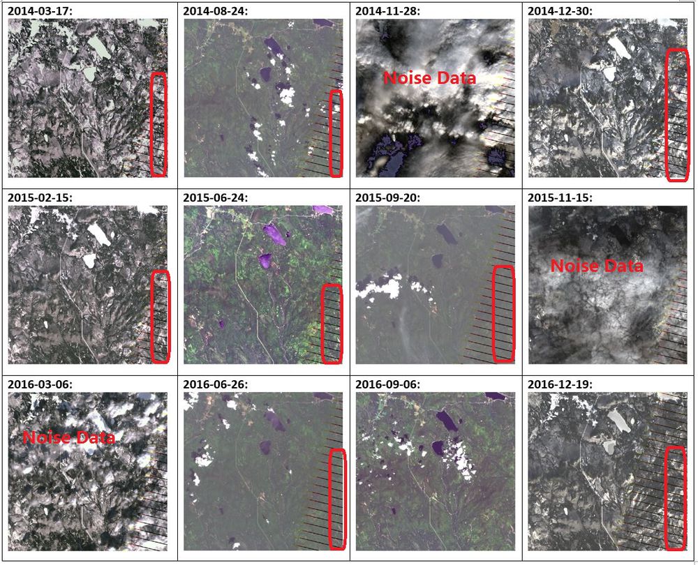
When looking at these "true-color" images, there are three images in which the preserve area cannot be seen clearly due to the clouds.
These three images are taken on 2014-11-28, 2015-11-15 and 2016-03-06.
As the clouds have covered more than 90% of the area in these images, I think they are meaningless to my further analysis.
Hence, I take the three images as noise data and they should be filtered out.
Besides, among the remaining nine images, I noticed that the image which was taken on 2016-09-06 is a little different from the others.
In the other eight images, there are many bad pixels in the right bottom corner due to sensor failure or electronic noise.
Compared to others, the image taken on 2016-09-06 is much more clear. It is a good choice to locate the position of the Boonsong Lake in the preserve.
Load Data into JMP
Concatenate Data
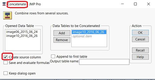
To compare the changes in different days, I concatenate the data in JMP as below. It will create one column as the "Source Table".
Add Date
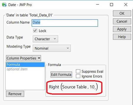
Then I add a column "Date", which shows the date of the image.
NVDI Calculation
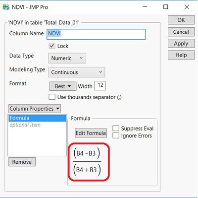
According to the definition of NDVI (Normalized Difference Vegetation Index): NDVI = (B4 - B3) / (B4 + B3), I add the formula to calculate the NDVI value.
Create Bins in Tableau
The bands are continuous measures. Any discrete field in Tableau can be considered as a set of bins.
In the Data pane, right-click a measure and select Create > Bins.
In the Create Bins dialog box, I entered 5 in the Size of bins field since the range of all the band values are between 0 and 255.
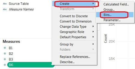
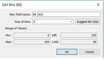
Then a new binned field appears in the Dimensions area of the Data pane.