Teppei Syokudo - Improving Store Performance: ESK Data Analysis Methodology
| Home | Product Portfolio Analysis | Improving Store Performance | Project Management | Documentation | The Team |
Data Exploration
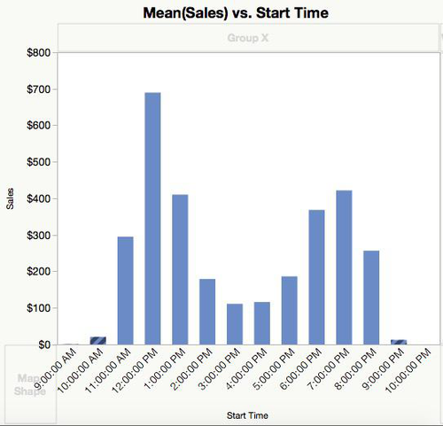
Time of Day Effect. We were provided with hourly and daily data for both sales and labour within a three month period. In exploring the data given, we found that there was a pattern in the sales transactions.
Mean sales per hour peaked from 11:00 to 13:00 and from 18:00 to 20:00. We attribute the peak periods to the lunchtime and dinnertime crowds respectively. Other time periods are idle time. We realise that this time of day effect will have to be taken into account when evaluating labour productivity in our hypotheses so that sales toward a particular factor would not be over or under attributed. We label 11:00 to 13:00 as Lunch Peak, 14:00 to 17:00 as Idle, and 18:00 to 20:00 as Dinner Peak.
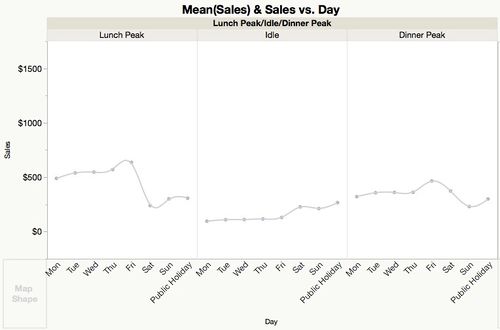
Day of Week Effect. We also found the mean sales for every day of the week. Accounting for the time of day effect, we find the mean sales each day of the week. The day of the week also accounts for public holidays as crowds may be higher during public holidays. Similar to the time of day effect, the chart below shows that there is also a day of week effect.
During Lunch Peak and Dinner Peak, the store tends to achieve higher sales average on Fridays, with Saturdays experiencing lower mean sales. However during Idle periods, Saturdays and Public Holidays tend to experience relatively better mean sales compared to Idle periods on other days in the week.
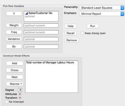
Removing Autocorrelation. We test for autocorrelation using the Durbin-Watson test. Taking the example for testing the effect of manager presence on sales per customer, we ran a Fit Model using Y as Sales/Customer Number and Model Effects using Total number of Manager Labour Hours.
The results of the Durbin-Watson test is shown below:
With p-value less than 0.05, we know that autocorrelation is present in our data. The Durbin-Watson value of 1.51 tells us that there is some positive correlation between Sales/Customer Number and Total number of Manager Labour Hours.
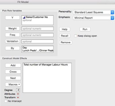
To account for the time of day and day of week effects, in the Fit Model, we add Day and Lunch Peak/Idle/Dinner Peak into By.
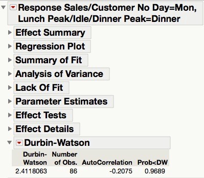
The results of the Durbin-Watson test this time is:
The p-value is greater than 0.05, showing that autocorrelation is no longer present in the data. We now know that for the analyses we run next, in order to account for the time of day and day of week effects, we should include Day and Lunch Peak/Idle/Dinner Peak in By.
Data Cleaning
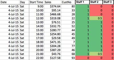
Our dataset comprises of 48 staff and their hourly labour records from 1st June 2015 to 31st December 2015. As the shop is opened seven days a week from 9:00am in the morning to 23:00 at night, we collected 2,996 hours’ worth of data over 214 days. The “Date” column indicates the date for each hourly data point, and the “Day” column indicates the corresponding day, from Monday to Sunday, as well as Public Holidays.
We allocated a number from 0 to 1 to each staff for his presence during each hour. For example, if the staff was present the full hour, he will be allocated a “1”. He will be allocated “0” for the hours that he was not present and “0.5” for the hours that he was present for only half the time.
Hourly store performance figures such as store sales (“Sales” column) and customer numbers (“CustNo” column) were also included after examining data from the POS system.
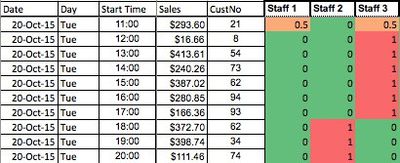
In addition, to test some of the hypotheses that we have thought of, we collected data on the staff that was manning the cash register for each hour (cashier data). The cashier data was then prepared in the same format as above. Cashier data was available from 20th October to 31st December.
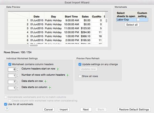
Both datasets were then imported into JMP using the “Open…” function.
After toggling the worksheet setting such that the column headers are correctly reflected, we can proceed with importing the data using the “Import” function.
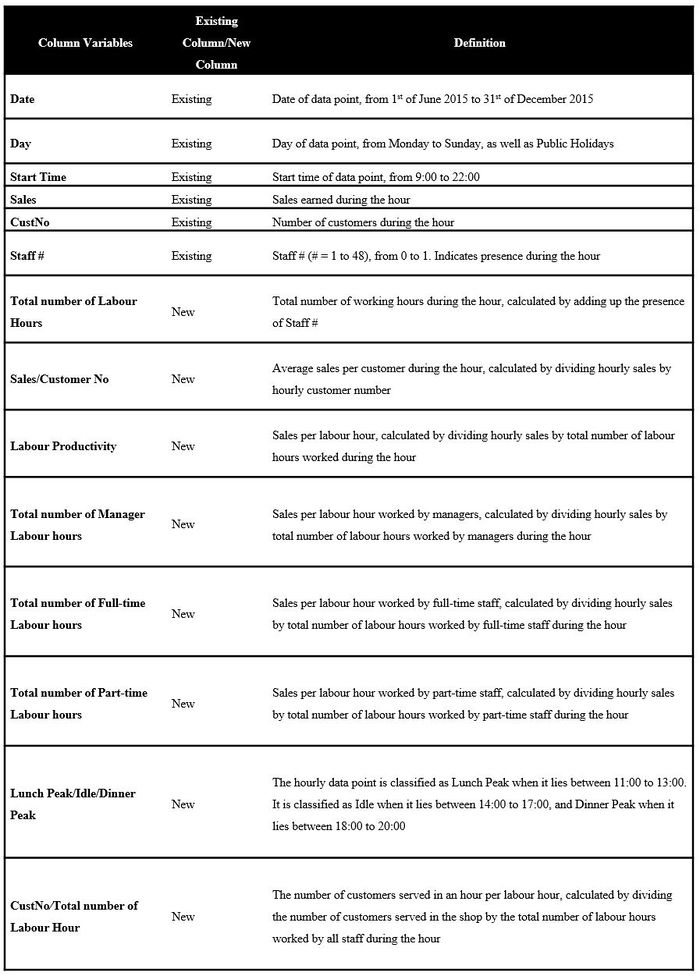
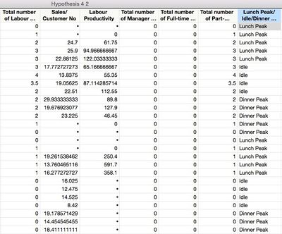
The following data table was then generated in JMP for further analysis. In order to test our hypotheses, we had to create new columns that were not included in the data set. All the column variables are indicated in the table below.
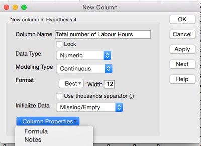
We added the new columns into the JMP table using the “Add new column” function. For example, we wanted to add a calculated column for “Total number of Labour Hours”
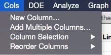
Step 1: Click Cols in the Menu Bar, then select New Column.
Step 2: Under Column Properties, select Formula.
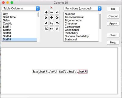
Step 3: Under Statistical, click on Sum, and then select Staff 1 to Staff 5
Step 4: Click Apply
We repeated this process for all the new columns to obtain respective calculated columns.
