ANLY482 AY2017-18T2 Group18/TeamDAcct Project Methodology
| Home | About Us | Project Overview | Project Findings | Project Management | Documentation | ANLY482 Homepage |
Data Preparation:
All the files acquired have helped us deepen our understanding of the company’s business and ultimately the business problem. However, not all files were crucial to formulate recommendations to the business problem on hand. The following are the list of data-sets prepared:
- Master Client Listing
- Facility Details
- Manpower Details
Following which, EDA (e.g. through the usage of graphs or tables of summary measures) was conducted to get a better understanding of the data. From the EDA, we will have a better understanding of the relationship amongst the explanatory variables (factors that drives the expenses such as wages) as well as provide us with a general direction and size of relationship between explanatory and outcome variables. In the analysis of data, we will be using the software SAS JMP Pro 13 as our main tool for data cleaning, data preparation and EDA. Our choice of this software is that it allows us to conduct statistical analysis on big datasets and can generate results that are easy to understand for end users. In addition, due to its popularity of being widely used, tutorials are readily available on the web, should we encounter any problem.
Thereafter, we can formulate and suggest a model to the client that forecast the expenses incurred for an anticipated project site with certain characteristics. From a business perspective, this would point to possible approaches management wish to take (i.e. minimise cost, bid at higher price, pegged to industry price, market share growth), in using our proposed model to assist in shortlisting future project sites and to drive business strategy overall.
After cleaning and preparing the data, we decided to work on our confirmatory analysis to assess the appropriateness of the explanatory variables to be used for our regression analysis. Thereafter, we performed multiple linear regression to build an explanatory model to analyse whether an increase in any of the explanatory variables (determined in our confirmatory analysis) has an impact on any of the various cost components incurred for a cleaning project type. The four major cost components that we have identified in a cleaning project are namely:
- Total Project Costs
- Manpower Costs
- Chemical & Materials Costs
- Equipment Costs
For this project, we will be focusing on one specific cleaning project type - conservancy sites (zones).
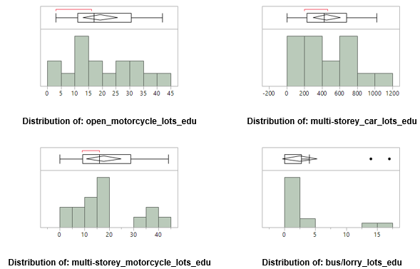
We first analysed the distribution of the explanatory variables identified (dwelling units, market/hawker stalls, commercial units, open car-lots, open motorcycle-lots, multi-storey car-lots, multi-storey motorcycle-lots, bus/lorry lots) that describe the attributes of conservancy zones. These are represented as shown:
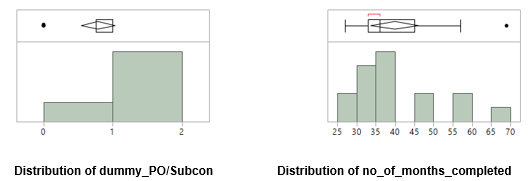
Upon closer inspection of the explanatory variables: market/hawker_stalls_edu and bus/lorry_lots_edu, it was found that majority of conservancy zones had zero market/hawker stalls and bus/lorry lots. We decided to categorise these numerical variables by putting the data into discrete categories (called bins). Dummy variables were introduced, where it is coded as 1 for all observations that had – for example, non-zero market/hawker stalls, and 0 for all observations that had zero market/hawker stalls.
The subsequent distribution of the above dummy variables introduced are represented as shown:
From our exploratory data analysis on conservancy project sites, we can see that for several of LS 2’s conservancy project sites that it undertakes, it engages third party (subcontractor) to perform under a subcontract all or part of the work that was included in the original contract won by LS 2. We decided to account for this by introducing a dummy variable, where it is coded as 1 for all observations that were performed in-house (i.e. not subcontracted out), and 0 for all observations that were not performed in-house (i.e. subcontracted out).
Additionally, as our cut-off period of interest for data collection was determined to be December 17, several of LS 2’s conservancy project sites as at that date were still in continuation. We decided to account for this by introducing an explanatory variable: no_of_months_completed, which provides the number of months underwent for all observations.
The subsequent distribution of the above variables introduced are represented as shown:
In addition, from our data preparation phase, we remarked that in general, conservancy contracts specify the minimum number of equipment they require LS 2 to deploy for the projects. We decided to account for this in our model that specifically analyse whether an increase in any of the explanatory variables identified (and introduced) has an impact on equipment costs. This was done by introducing three explanatory variables: minimum_battery_operated_cart, minimum_high_pressure_washer, minimum_hot_high_pressure_washer. From inspecting the table of datasets of ‘Tab 1: List of inspection unit’ prepared in ‘Facility Details (Conservancy)’, we selected these column names and screened the data by performing exploration for missing values. This was due to a few conservancy contracts not specifying the minimum number of equipment required to be deployed. Thereafter, the missing values were replaced via multivariate normal imputation, using the least squares prediction from the non-missing variables in each row.
The subsequent distribution of the above variables introduced are represented as shown:
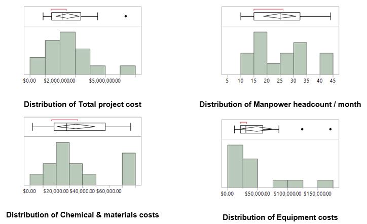
We also analysed the distribution of the dependent variables identified to check for skewness. These are represented as shown:
Multiple linear regression (MLR) is an approach for modelling the relationship between a scalar dependent variable y and more than one explanatory variable denoted xi. MLR allows us to use more of the information available to estimate the dependent variable. The best MLR model accounts and explains for the largest proportion of the variation in the dependent variable, with the fewest number of independent variables.
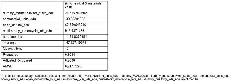
In each of our four models built, the procedures were as follows: We first looked at pairwise correlations among the explanatory variables determined. This is to check whether a high linear dependency exists among pairs of predictors. (Refer to Appendix 6.0 for details of correlation tests on all models) Thereafter, using SAS JMP we constructed the MLR model via standard least squares method that minimises the sum of squared errors. Effect screening was performed to verify the significance of each explanatory variable. Using the p-value of t-test as a rule of thumb in assessing the statistical significance of the explanatory variables, variables with p-value >= 0.05 (denote that the variable is insignificant in the model, at a 5% significance level) are removed one-by-one. We also check for presence of multicollinearity , and variables with high VIFs detected (VIF > 10) are subsequently removed. The model is re-computed each time to arrive at a final equation. The results of the regression model are shown in Figure 27 and Figure 28 represented below.
We also constructed the MLR model via step-wise method that is carried out by an automatic procedure. Two main approaches, Forward Selection and Backward Elimination were performed and the automated model was run (Refer to Appendix 7.0 and 8.0 for details on Forward Selection and Backward Elimination Results in all models, respectively). For forward selection, we specified a p-value threshold of 0.25 as the model fit criterion to allow the variable to enter the model. For backward elimination, we specified a p-value threshold of 0.05 as the model fit criterion to allow the variable to stay in the model.
Comparing the results of our manual model to both the forward selection and backward elimination approach (as shown in Figure 29-32 below), we observed that for Model (i) and (iii), backward elimination gives similar results (in terms of Final equation) to our manual model. Across all models, we considered the adjusted R-squared value as a rule of thumb in assessing whether forward selection or backward elimination, compared to the manual model, provides an improved model result. Ultimately, the manual model was preferred over forward selection and backward elimination approaches. This was because even though the approaches yielded a higher adjusted R-squared value, it did not remove variables with high VIFs detected.
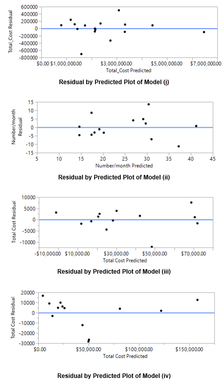
Next, we reviewed the overall model significance to ensure goodness of fit. Using the p-value of f-test as a rule of thumb in assessing the overall fit of the regression model, a p-value of <0.05 indicates the model is significant (at a 5% significance level) in predicting the dependent variable better than its mean value. All models were ascertained to have p-values <0.05. Finally, we verified that the assumptions in multiple linear regression were respected by using the residuals plot to ensure that the errors are randomly distributed. The subsequent residuals vs. predicted value plot for model (i), (ii), (iii) and (iv) are represented as shown:
