ANLY482 AY2016-17 T2 Group3: HOME/Final
| HOME | ABOUT US | PROJECT OVERVIEW | PROJECT FINDINGS | PROJECT MANAGEMENT | DOCUMENTATION | ALL PROJECTS |
Contents
Update
Moving forward from the Interim, our team has continued our analysis. The following will show our progress and findings from the Cluster Analysis and Association Analysis that we carried out. For better understanding on the entire project, you may look at our Final Research Paper. Thank you!
Cluster Analysis
Clustering Variables
After getting a clearer picture of the dataset through Exploratory Data Analysis, the next analysis that we will focus on is Cluster Analysis. The purpose of this analysis is to identify and segmentize current customers into distinct clusters of varying characteristics. First and foremost, we had to identify potential clustering variables from the Users table. After analyzing Users table, we felt that the existing variables such as age and gender was not very suitable to be used in clustering. The age range was not very wide and customers were predominantly female.
Hence, we decided to utilize the 3 variables from the RFM analysis and generate the columns shown in Figure 1 above for each customer. However, only customers with at least 1 booking were considered to ensure that the clusters formed were distinct enough. For booking_recency, it refers to the number of weeks since the customer’s last booking with respect to 31 December 2016. In terms of the monetary variable, the total monetary value of all the customer’s bookings is used instead as average monetary value is not very indicative of how much the customer had spent in the last 2 years.
Next, before commencing K-Means Clustering, it is important to understand the distribution of the 3 variables. A variable that is highly skewed will have to be normalized as K-Means Clustering is highly susceptible to such noise and outliers.
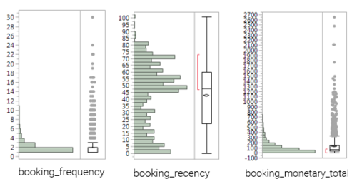
Based on Figure 2 above, booking_frequency and booking_monetary_total are highly right-skewed while booking_recency is still relatively normal. Hence, for 2 variables with a skewed distribution, a log10 transformation was used in an attempt to balance the distributions and make them more normal.
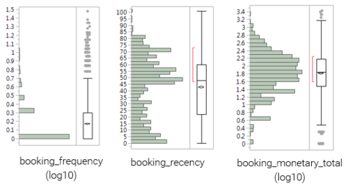
After applying the log10 transformation, the revised distributions are shown in Figure 3. Interestingly, the transformation only managed to successfully normalize the distribution of booking_monetary_total while the distribution of booking_frequency remained largely right-skewed. This was most probably due to the fact the monetary values were more continuous as compared to the frequency which seemed more discrete. Hence, we selected the initial values of booking_frequency and booking_recency as well as the transformed values of booking_monetary_total for the clustering.
Clustering Results
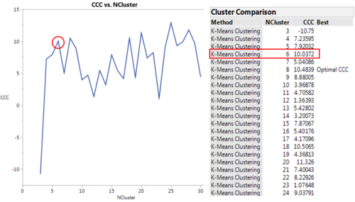
To conduct the clustering, we have utilized the in-built K-Means CLustering function found under “Multivariate Methods” in JMP Pro. However, before kickstarting the K-Means Clustering, the number of clusters had to be decided. By customizing and setting the number of clusters to range from 3 to 30, we obtained the graph shown in Figure 4 which plots the Cubic Clustering Criterion (CCC) against the number of clusters. CCC values are similar to R Squared values that basically indicate the optimal number of clusters to form. In general, the idea is to identify the point where the CCC to increase to a maximum and starts to decrease. At that point, we would then take the number of clusters as the optimal value. In this case, the optimal number of clusters to form is 6.
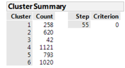
After running K-Means Clustering with and intended number of clusters set to 6, we managed to get 6 different clusters of varying counts as well as their cluster means (as seen in Figure 5 and Figure 6). At a glance, the number of customers in each cluster seem to be relatively uneven, especially in cluster 3 where there are only 42 customers present. We will look into this unique cluster and its characteristics when we profile each cluster accordingly below.
For the profiling of clusters, we have generated the Parallel Coordinate Plot for each respective cluster. This plot basically gives a more visual representation of any patterns that may arise within the cluster itself. More specifically, each clustering variable is a column with its binned range of values displayed vertically. Color-coded polylines are then drawn and the range of values the cluster contains for every variable are shown. Ideally, each cluster should have a profile that is distinct enough from other clusters.
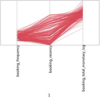
For cluster 1, the general shape of plot is relatively dense, giving the cluster distinct and unique characteristics (as shown in Figure 7). Even though this cluster only contains 258 customers, there is an average booking frequency of 6 and a decently high average total monetary value of $125. The only visible drawback is its widespread booking recency, which means that while there are customers that booked quite recently (within 1 month) there are also customers that have not booked in a while (6 months). This may imply that customers within this cluster were actually making bookings regularly and spending decently but may have stopped this behaviour in recent months.
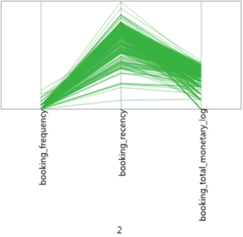
For cluster 2, the general shape of plot is also relatively dense, giving the cluster distinct and unique characteristics (as shown in Figure 8). As compared to cluster 1, this cluster has a higher number of customers (620). However, all 3 clustering variables are not too desirable where customers have only booked once, not very recently and are not willing to spend much on beauty services (average total monetary value of only $12). This seems to suggest that customers within this cluster are slowly dropping of from using the beauty application entirely.
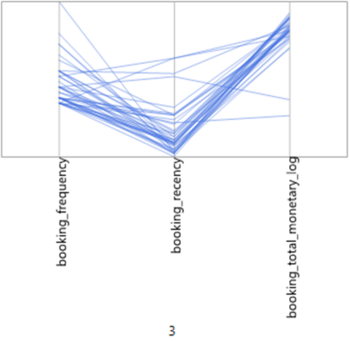
For cluster 3, as mentioned earlier, it only has 42 customers which is relatively intriguing (as shown in Figure 9). As compared to the previous 2 clusters, the shape of the cluster is understandably more sparse. However, customers within this cluster fare exceptionally well when it comes to the 3 clustering variables. There is high frequency, low recency (within 2 to 3 months) and a high average total monetary value of approximately $700. Although the number of customers within the cluster are low, this cluster could potentially represent Vanitee’s high valued group of customers that could be targeted differently.
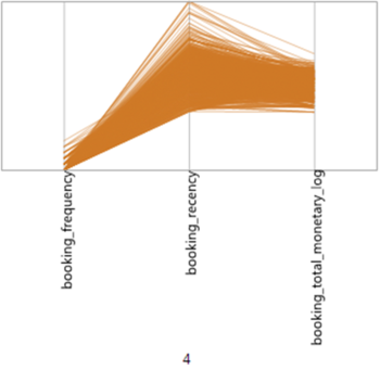
For cluster 4, the general shape of plot is also relatively dense, giving the cluster distinct and unique characteristics (as shown in Figure 10). As compared previous clusters, this cluster has a higher number of customers (1121). Unfortunately, majority of customers within this cluster have only booked once and have not booked within the last 4 months. The only upside is that they have spent an average total monetary value of $60 in their first booking which indicates that they are willing to spend but are somehow not making more bookings.
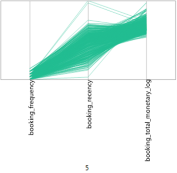
For cluster 5, the general shape of plot is also relatively dense, giving the cluster distinct and unique characteristics (as shown in Figure 11). This cluster has approximately 793 customers. Its shape is relatively similar to cluster 4 in terms of its low booking frequency. However, the booking recency of customers within this cluster is more widespread and customers are willing to spend much more on beauty services (average total monetary value of $238).
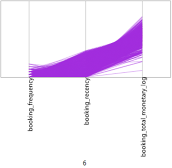
Lastly for cluster 6, the general shape of plot is also relatively dense, giving the cluster distinct and unique characteristics (as shown in Figure 12). This cluster has approximately 1020 customers. Its shape is relatively similar to clusters 4 and 5 in terms of its low booking frequency. However, the booking recency of customers within this cluster is slightly lower and customers are willing to spend a medium amount (more widespread) on beauty services (average total monetary value of $89). Clusters 4, 5 and 6 are relatively similar and may be indicate of the mass market where most customers have only booked once even though they are willing to spend on beauty services.
Association Analysis
The last analysis that we will be focusing on is Association Analysis. As mentioned earlier, the main purpose of this analysis is to better understand customers booking behaviour. Before conducting this analysis, there are a couple of technical terms that have to be defined first. Association Analysis basically tries to uncover any potential association between Items with the same Transaction ID. In this case, Item refers to the specific category of a service (e.g. nails, makeup etc.) that the customer includes in a booking. Transaction ID refers to the ID of the transaction that the item belongs to (i.e. the ID of the booking).
Currently, the Bookings table is structured in a way where each row is a booking record and each record can keep track of multiple service IDs to indicate the services that the customer has selected (as seen in Figure 13). However, this does not fit the requirement to conduct Association Analysis as it is impossible to derive any association rules this way. Hence, the data in the Bookings table had to be transposed in a way where each service ID forms an entirely new row on its own. Looking at Figure 14, the 2nd and 3rd row are actually services that belong to the same booking. After transposing the data, the level 1 category of the service (category_1) is generated for each row. The level 1 category refers to the master categories that Vanitee had defined, meaning that they are more generic in nature. In the later part of this section, we will look into whether this category_1 variable’s suitability as the Item in Association Analysis.
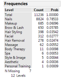
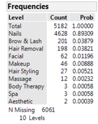
The next issue faced was whether bookings with only 1 service should be included in the analysis. Understandably, these bookings will cause the results to weaken as no association can be drawn from just 1 service within the booking. However, we wanted to see if there were any huge difference in the analysis if we were to include or exclude these bookings. Figures 15 and 16 above show the frequency distributions of the category_1 variable including and excluding bookings with only 1 service respectively. Interestingly, both actually show that there is way more bookings that have included nail services as compared to the other service types. This is primarily due to the fact that there are much more nail services offered on this platform as seen in the EDA section earlier.
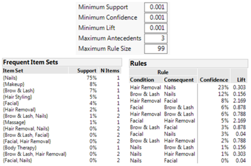
Next, we utilized the Association Analysis platform under “Screening” in JMP Pro to customize a few parameters (as seen in at the top of Figure 17). Support refers to the proportion of transactions in which a specific item set appears. Confidence refers to the proportion of transactions that contain the consequent item set given that the condition item set is in the transaction. Lift refers to the ratio of an association rule’s confidence to its expected confidence. In general, the higher the value in these 3 variables, the more insightful the association rule is. However, in this analysis, we have set these variables to a minimum of almost zero, in an attempt to discover all association rules.
The bottom 2 tables in Figure 17 show the results of the analysis when bookings with only 1 service are included. The left table depicts the frequent item sets that occur while the right table states the association rules that have been found. For example, the {Nails} item set has a support of 75%, meaning 75% of the bookings have a nail service included. However, we can see that the support for the rest of the item sets are significantly lower. For the association rules, we can see that the first rule states that with the condition as ‘Hair Removal’ and consequent as ‘Nails”, the confidence is only 23% with a lift of 0.303. For it to be insightful, the confidence should be at least 50% and the lift should be more than or close to 1. Hence, we can observe that the results of this analysis are relatively insignificant.
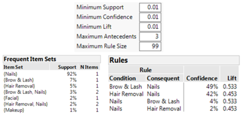
On the other hand, the analysis was rerun where bookings with only 1 service were excluded to see if better results could be obtained. A quick glance at the rules generated in Figure 18 show an improvement in the confidence and lift of the rules. Specifically, when we zoom into the first rule with ‘Brow & Lash’ as the condition and ‘Nails’ as the consequent, we observe a confidence of 49% and lift of 0.533. However, when we look at the condition, ‘Brow & Lash’, in the frequent item sets table, we noticed that its support is at a low value of 7%. This means that this rule may only be true 7% of the time.
Moving on, we decided to understand the potential reasons for the unsatisfactory results. As mentioned earlier, the results may have been affected due to the high frequency in the number of nail services, whether bookings with 1 service were included or excluded. Upon closer inspection, we realized that this high frequency resulted from the way the level 1 categories were classified. As shown in Figure 19, the services in the first 3 rows belong to the same booking. However, all of them were classified to be under Nails, which means that in this booking, there are no “difference” in the categories of services included. Hence, we deduced that the category_1 values are perhaps overly generic to be used in Association Analysis.
Eventually, we decided to breakdown each level 1 category into its level 2 category (category_2) which are categories that are still defined by Vanitee but are much more specific in nature. For example, looking at Figure 20, the ‘Nails’ category can be split into ‘Gel’ and ‘Nail Art’ while the ‘Hair Styling’ category can be further categorized into ‘Colour’ and ‘Cut’. In this case, we can be certain that there are at least bookings with a differentiated number of services included.
Next, we applied the same methodology and ran the same analysis, starting with including bookings with only 1 service. As expected, there was a huge improvement in the results, especially in the association rules generated. As seen in Figure 21, most of the association rules have a lift that is close to 1 and some of them have a confidence close to or more than 50% (as highlighted by the red box). However, we noticed that there was the same issue of low support for the condition in the association rule. For example, the rule with ‘Nail Art, Removal’ as the condition and ‘Classic’ as the consequent has a healthy confidence of 61% and lift of 1.524. However, when we look at the condition, ‘Nail Art, Removal’, in the frequent item sets table, its support is at an extremely low value of 2%. This means that this rule may only be true 2% of the time which is highly insignificant.
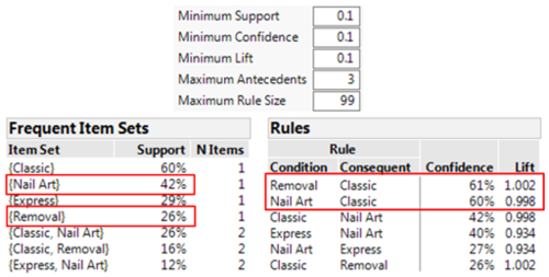
Lastly, we decided that the previous issue was brought about by including bookings with only 1 service. Hence, the analysis was run again but this time bookings with only 1 service were excluded. Looking at Figure 22, the results generated are largely encouraging where the support of the condition in the association rules are largely adequate. For example, the rule with ‘Nail Art’ as the condition and ‘Classic’ as the consequent has a healthy confidence of 60% and lift of 0.998. Furthermore, the ‘Nail Art’ has a decent support of 42%. To put it in words, we can state that 60% of customers that include a ‘Nail Art’ service, will be likely to include a ‘Classic’ service within the same booking. Also, this is going to be rather prevalent where there are already 42% of existing bookings that have a ‘Nail Art’ service.
However, we do acknowledge some of the limitations posed by the behaviour of actual customers and professionals. For example, customers tend to engage in services that are related to each other (e.g. within nails category itself) instead of engaging in two distinctively different services (e.g. nails and facial). Furthermore, professionals usually offer services that they specialize in (e.g. a nail artist does not do hair styling).
Through this analysis, we got to dive deeper into understanding the way customers go about making their bookings. Even though the rules generated may be obvious, they still give an insightful view as to what is the exact percentage that a specific rule is true.
Recommendations
The analyses and findings have shown us that there are effectively different groups of customers that are using Vanitee’s beauty platform. As such, marketing efforts targeted at these groups should be differentiated to suit characteristics and purchasing behaviour of each group. Looking at the results from the Cluster Analysis, a recommendation we have is a one time offer for the group of customers that have been dormant (i.e. clusters 4, 5 and 6) so as to entice them to make another booking. After all, these group of customers are willing to spend an average amount on bookings. Also, another distinct group of customers we saw is the niche market group (cluster 3) who are willing to spend more than the average on a frequent and recent basis. For this group, Vanitee can look at promoting packaged offers to them to attract them to take up more services in their next bookings. Moving forward, Vanitee should start keeping track of the three variables from the RFM model to analyse customer behaviour in future.
Through Association Analysis, association rules have been derived to show the correlation between that certain services that are typically purchased together in a single booking. Understanding that there is a strong association between ‘Nail Art’ services and ‘Classic’ services, Vanitee can convey these information to their beauty professionals so that they could offer bundled beauty services that include the 2 mentioned services. On the other hand, Vanitee can create campaigns that are tailored to these 2 types of services where discounts can be enjoyed only if the booking contains both service types. This would encourage customers to not only book more frequently but also purchase more services within a single booking.
Lastly, Vanitee can also make use of Association Analysis to determine the popularity of a new level 2 category. Since the analysis is able to state the support and deduce association rules, it would be possible to look at whether a new category is effective in satisfying the customers taste and preferences. Furthermore, Vanitee can work on their level 3 categories to introduce more specific categories and utilize this analysis to see its effects.
Conclusion
At the start of this paper, we set out to understand more about Vanitee’s business and its customers by targeting the Acquire and Enhance phases of CRM. Having understood the general profile of their customers and their booking behaviour through Exploratory Data Analysis and RFM analysis, we observed the platform does facilitate the demand and supply for beauty services. However, even with customers on board, many of them have only booked once and the recency of their booking varied over a large range. Hence, we proceeded to carry out Cluster Analysis in an attempt to segmentize their customers into 6 clusters with distinct characteristics by using the 3 variables in the RFM analysis. Thereafter, we were able to profile these clusters accordingly and provide a more visual representation to Vanitee’s existing customers.
Lastly, we ended with Association Analysis which provided a clearer picture as to how customers select different types of services within a single booking. All in all, we hope that Vanitee would be able to use the insights from this paper to continue improving their business and provide this platform for independent beauty professionals and customers in Singapore.


