ANLY482 AY1516 G1 Team Skulptors - Outbound EDA
![]()
| Data Cleaning new! | Inbound EDA new! | Outbound EDA new! |

Regarding the outbound data, there are limitations on the analysis on the pick rate of the warehouse stock. For example, in our inbound, we are largely concerned with the pallets inbound (Warehouse stores items in pallets). However, for outbound, the company is more concerned about the quantity of outbound. This is because not all warehouse outbound movements are large quantities. For instance, a company might only need 50 pieces syringes instead of a carton to top up their medical kit.
Regarding the outbound data, there are limitations on the analysis on the pick rate of the warehouse stock. For example, in our inbound, we are largely concerned with the pallets inbound (Warehouse stores items in pallets). However, for outbound, the company is more concerned about the quantity of outbound. This is because not all warehouse outbound movements are large quantities. For instance, a company might only need 50 pieces syringes instead of a carton to top up their medical kit.
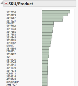
For outbound, popularity of SKUs/products is very important as they influence the inbound rates of the product. For instance, if a certain product is fast moving, it shows that the product is popular and thus, more inbounds are required to satisfy the demand. Popularity of the product can in turn predict the movement of the product, which is information useful to the warehouse manager. He or she can then allocate spaces accordingly for the popular or unpopular products. The team has sorted the outbound frequency of the SKUs/products in descending order.
From the distribution analysis above, we can see that the top 4 products accounts for much difference compared to the outbound movements for other products. There is a high possibility that the first 3 digits (361) is used to depict popular product as they most products which are in the top few spots of the bar chart generally share the same 361 prefix. In the bar chart above, we can notice that the top 10 SKUs are mostly products with product codes that starts with 361.
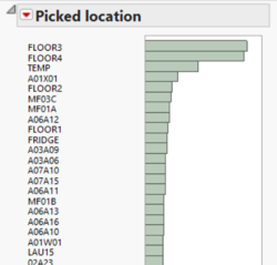
Similar to the inbound data, the top picking location where the stock is being picked up from, revolves around the FLOOR or the TEMP location. However, one point to note would be the most popular location. In the inbound, majority of the product stock keeping units are stored in the TEMP location, which our team believes is the temporary location. But in this graph, instead of TEMP being the most popular location for picking, it is the floor areas namely, FLOOR3 and FLOOR4 instead. A distinct problem and discrepancy can be identified here as most of the inbounds are stored at the TEMP location however, most of the outbound is picked from the FLOOR locations. Hence, there would be high possibility that there would be a problem of overflowing over at the TEMP location. This issue will this, require further investigation and clarification with the client. As for the other pick locations, they are generally quite even in terms of picking rates. Nonetheless, the team believes that picking could be utilized and done better since most of the pick location revolves around the FLOOR and TEMP locations.
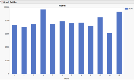
In this graph, our team looks at the distribution of the outbound on a monthly basis. There is a general consistency in the outbound, with a minimum of 6122 in November 2015 (Month 11) and a maximum of 9654 in the April 2015 (Month 4). However, this graph is limited in a sense it only shows outbound frequency by monthly basis. For instance, it is unable to show the volume of outbound – i.e. a month might have very little outbound, but each outbound is a large outbound of more than 1 million pieces. Nonetheless, it is still useful in providing a general overview to the clients. This is also because based on our previous findings, the team had noticed that the pick rate mean and bound is relatively consistent. Hence, each outbound is roughly identical in outbound size.
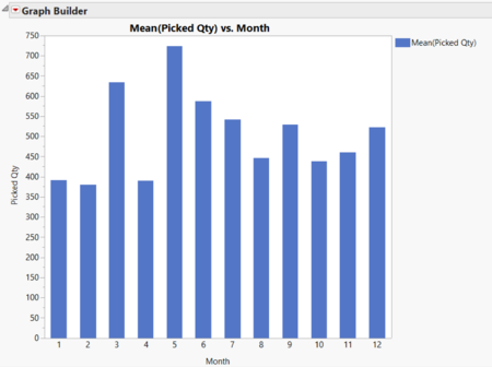
To investigate on the volume scenario, the team plotted a bar chart with y-axis consisting of picked quantity versus the x-axis time dimension, month. Here we can see the average picked quantity of outbound in each month, which shows much more variation as compared to the previous graph. These two graphs can be used hand in hand to show volume of outbound. As mentioned earlier, the outbound is limited due to the use of measurement – pieces versus pallets. The number of pallets consumed is not shown in the outbound data. Hence, the team’s analyzation is only restricted to pieces. In addition, from a warehouse point of view, a unit measure of different products can be vastly different in space occupation. For instance, a syringe and an alcohol swab is both 1 unit of measure in piece however, an alcohol swab is definitely much smaller compared to a syringe.
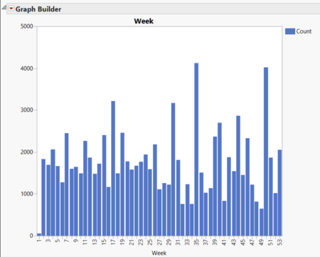
This graph further slices the time dimension to a weekly level analysis. Through it, we can see generally in each week, there is at least one outbound. However, there is a shockingly vast differences in outbound rates for each week in the 2015 working year. For instance, it can go as low as 61 times in the first week to 4060 times in week 35. This is cost-heavy and taxing on the warehouse employees as warehouse employees have to cater to this fluctuations which are relatively volatile. This can be seen from the graph above, where the outbound rate jumps around at random from high to low and vice-versa. Ideally, with proper planning, the outbound rates can be relatively consistent and controlled. There are two scenarios that can help warehouse employees:
1. Periodic outbound: Outbound rates are pushed seasonally so warehouse employees will know when to account for high and low pick rate periods
2. Consistent outbound: If outbound rate is kept relatively constant and within control, it is much easier for the warehouse to prepare for these outbound
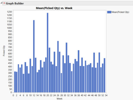
Similar to before, the team included the picked quantity in the y-axis versus the x-axis time dimension, week. The variations are similar to the pick rate count in the previous graphs, but in terms of average picked quantity, they are still more controlled than before, with the exceptions week 12 and week 20. These two weeks peaked the mean picked quantity, exceeding a thousand quantity picked in a given week. This graph can be used hand in hand with the previous graph to show the volume of outbound rate on a weekly basis.
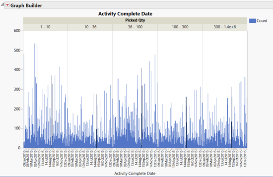
In this graph, the team wanted to see the dates where each group of picked quantity is commonly found in. Hence, the team segregated the picking quantity into 5 categories, 1-10, 10-36, 36-100, 100-300, and more than 300. The reason why the groups are not uniform in picking quantity size are because these picking sizes are packaged in such a way that anything less than 10 pieces is taken loosely. 10-36 will be in a box, 100-300 will be in a carton, while anything more than 300 will need to be in a pallet etc. These segmentation will give a better representation of the frequency of different quantity outbound. Based on the graph, we can see that all categories have a healthy consistency, with 1-10 picked quantity ranging slightly more. A peculiar fact that can be helpful to the company is the Activity Complete Date (Day where the goods are picked). Other than the 1-10 category, all other categories are more common in the later portion of the year.