Difference between revisions of "ANLY482 AY2016-17 T2 Group23 Silver Daisies Analysis and Findings"
| (43 intermediate revisions by 2 users not shown) | |||
| Line 1: | Line 1: | ||
| − | |||
| − | |||
| − | |||
| − | |||
<!------- Main Navigation Bar----> | <!------- Main Navigation Bar----> | ||
| Line 29: | Line 25: | ||
<!------- End of Main Navigation Bar----> | <!------- End of Main Navigation Bar----> | ||
| − | == | + | == Univariate Analysis == |
| − | + | === Appointment Duration === | |
| + | We performed univariate analysis on appointment duration to find out the current distribution and summary statistics and obtained the following results: | ||
| + | [[File:Duration.png|700px|frameless|none]] | ||
| + | |||
| + | * Mean duration: 1:22 | ||
| + | * Median duration: 1:12 | ||
| + | * Standard deviation: 0:47 | ||
| + | * Non-parametric distribution | ||
| + | |||
| + | == Bivariate Analysis == | ||
| + | We performed bivariate analysis on each independent variable to find out their individual effect on appointment duration and obtained the following main findings: | ||
| + | |||
| + | ===Appointment Clinic === | ||
| + | The median duration differs from clinic to clinic. The longer average appointment duration includes SNEC (Singapore National Eye Center), NUH (National University Hospital), and NCC (National Cancer Centre). The shorter durations mainly come from neighborhood polyclinics, such as Geylang polyclinic, BMP (Bukit Merah Polyclinic), and CWC (Community Wellness Centre). | ||
| + | [[File:Appt clinic.png|400px|frameless|none]] | ||
| + | ===Appointment Purpose=== | ||
| + | From the distribution analysis, we can see that Ophthalmologist takes the longest duration while Tests takes the shortest duration. | ||
| + | [[File:newmed.png|400px|frameless|none]] | ||
| + | Through our median test of significance, we observed that blood test (non-fasting) is significantly shorter than blood test (fasting). | ||
| + | [[File:BT.jpg|300px|frameless|none]] | ||
| + | |||
| + | ===Escort=== | ||
| + | Analyzing the appointment durations when there is Next-of-kin accompaniment vs Family (more than 1 NOK) accompaniment vs Medical escort accompaniment, we see a difference in median appointment durations. We conducted a non-parametric paired significance test and conclude that with the accompaniment of a medical escort, the median appointment duration is lower than the accompaniment of NOK or family. | ||
| + | |||
| + | [[File:Escort.PNG|400px|frameless]] | ||
| + | |||
| + | [[File:TestEscort.PNG|700px|frameless]] | ||
| + | |||
| + | ==Multivariate Regression== | ||
| + | ===Stepwise Regression=== | ||
| + | As we have many independent variables and sub-variables, we will perform a stepwise multiple linear regression to select the relevant variables. The results also reveal how the partition splits are done. | ||
| + | [[File:Boxcox.png|400px|frameless|none]] | ||
| + | Based on Box-Cox Transformations, the y variable (appointment duration), is transformed based on the suggested lambda value of 0.263. After which it is transformed again by 0.986, before reaching a suggested lambda value of 1.0, which signifies that no transformation is needed. The Residual by Predicted Plot is now show as below. | ||
| + | [[File:residualbef.png|400px|frameless|left]][[File:residualaft.png|400px|frameless|none]] | ||
| + | |||
| − | + | ''<center><small><small>Residuals before transformation (left) and after transformation (right)</small></small></center> | |
| − | + | '' | |
| − | == | + | ===Durbin-Watson Autocorrelation Test === |
| − | + | [[File:Autotest.PNG|400px|frameless|none]] | |
| + | Based on Durbin-Watson Test, there is no significant evidence to conclude that the model is autocorrelated. | ||
| − | + | === Model Fit === | |
| − | |||
| − | + | [[File:Modelfit.PNG|400px|frameless|none]] | |
| − | + | The Summary of Fit shows a R-square of 0.318, meaning that 31.8% of the relationship can be explained with the given parameters. The adjusted R-square is 0.311, which is only a little lower than R-square, showing little evidence that the model is overfitted. | |
| − | + | [[File:Lackoffit.PNG|400px|frameless|none]] | |
| + | This is further supported by the high p-value in the Lack of Fit analysis. A high p-value shows that the model is close to being a saturated model. There is a 43.7% probability that this model can still be improved to a maximum R-square of 0.526. This usually means that exploration on a combination of variables is required. | ||
| − | + | [[File:Predplot.PNG|400px|frameless|none]] Due to the nature of having many categorical variables, the points are very spread out vertically. Although the prediction is not that reliable, there is no obvious visible evidence that it is not following a linear regression model. | |
| − | [[File: | ||
| − | |||
| − | === | + | === Recursive Partitioning === |
| − | [[File: | + | Recursive partioning was performed on the independent variables purpose and clinic as there are many sub-variables. [[File:Decisiontree.PNG|200px|frameless|right]] |
| − | |||
| − | + | Based on the above results that show the number of splits required, all the variables are recoded into ordinal variable based on their mean durations. Other independent variables can also be coded into ordinal variables based on their relationship with the response variable. The reduction of factor allows exploration of combination of x variables to produce a better predictive model. | |
| − | |||
| − | === Analysis | + | === Interaction Analysis === |
| − | + | A few variables were combined and permutated, adding them 1 by 1 to test whether the adjusted R-square increases. | |
| − | + | ||
| − | + | [[File:Varimp1.PNG|400px|frameless|none]] | |
| − | + | Based on the variable importance analysis, Ordinal Clinic*Ordinal Purpose explains 96.6% of the relationship. In terms of practicality, the user can simply look at the LS Means Plot of this variable to get a quick gauge of the appointment duration. | |
| + | |||
| + | However, based on the LS Means plot, we can see there are some levels with a rather high standard error. It will be less accurate in the prediction for level 16, 25, 32 and 40 but more accurate for other levers. | ||
| + | [[File:Varimp2.png|400px|frameless|none]] | ||
| + | |||
| + | Analysing the LS Means Plot of Ordinal Escort*Ordinal Walkability allows us to visualise that only level 3 seems to have the greatest impact on duration. This level 3 can only be achieved by the combination of Family being the escort, escorting the client in a wheelchair. From this, it is evident that family escorts tend to take a longer moving time with their wheelchair bounded family member. | ||
| + | [[File:Varimp3.png|400px|frameless|none]] | ||
Latest revision as of 02:16, 9 April 2018
Contents
Univariate Analysis
Appointment Duration
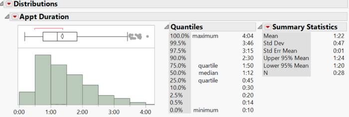
We performed univariate analysis on appointment duration to find out the current distribution and summary statistics and obtained the following results:
- Mean duration: 1:22
- Median duration: 1:12
- Standard deviation: 0:47
- Non-parametric distribution
Bivariate Analysis
We performed bivariate analysis on each independent variable to find out their individual effect on appointment duration and obtained the following main findings:
Appointment Clinic
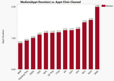
The median duration differs from clinic to clinic. The longer average appointment duration includes SNEC (Singapore National Eye Center), NUH (National University Hospital), and NCC (National Cancer Centre). The shorter durations mainly come from neighborhood polyclinics, such as Geylang polyclinic, BMP (Bukit Merah Polyclinic), and CWC (Community Wellness Centre).
Appointment Purpose
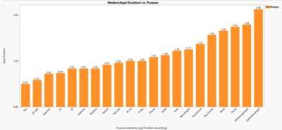
From the distribution analysis, we can see that Ophthalmologist takes the longest duration while Tests takes the shortest duration.
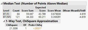
Through our median test of significance, we observed that blood test (non-fasting) is significantly shorter than blood test (fasting).
Escort
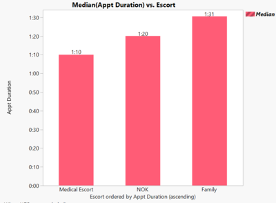
Analyzing the appointment durations when there is Next-of-kin accompaniment vs Family (more than 1 NOK) accompaniment vs Medical escort accompaniment, we see a difference in median appointment durations. We conducted a non-parametric paired significance test and conclude that with the accompaniment of a medical escort, the median appointment duration is lower than the accompaniment of NOK or family.
Multivariate Regression
Stepwise Regression
As we have many independent variables and sub-variables, we will perform a stepwise multiple linear regression to select the relevant variables. The results also reveal how the partition splits are done.
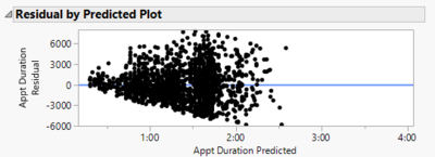
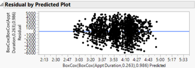
Based on Box-Cox Transformations, the y variable (appointment duration), is transformed based on the suggested lambda value of 0.263. After which it is transformed again by 0.986, before reaching a suggested lambda value of 1.0, which signifies that no transformation is needed. The Residual by Predicted Plot is now show as below.
Durbin-Watson Autocorrelation Test
Based on Durbin-Watson Test, there is no significant evidence to conclude that the model is autocorrelated.
Model Fit
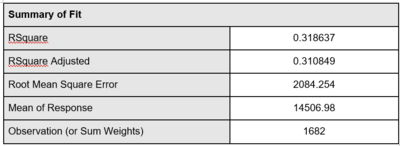
The Summary of Fit shows a R-square of 0.318, meaning that 31.8% of the relationship can be explained with the given parameters. The adjusted R-square is 0.311, which is only a little lower than R-square, showing little evidence that the model is overfitted.
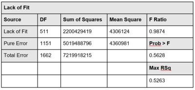
This is further supported by the high p-value in the Lack of Fit analysis. A high p-value shows that the model is close to being a saturated model. There is a 43.7% probability that this model can still be improved to a maximum R-square of 0.526. This usually means that exploration on a combination of variables is required.
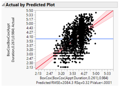
Due to the nature of having many categorical variables, the points are very spread out vertically. Although the prediction is not that reliable, there is no obvious visible evidence that it is not following a linear regression model.
Recursive Partitioning
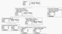
Recursive partioning was performed on the independent variables purpose and clinic as there are many sub-variables.
Based on the above results that show the number of splits required, all the variables are recoded into ordinal variable based on their mean durations. Other independent variables can also be coded into ordinal variables based on their relationship with the response variable. The reduction of factor allows exploration of combination of x variables to produce a better predictive model.
Interaction Analysis
A few variables were combined and permutated, adding them 1 by 1 to test whether the adjusted R-square increases.
Based on the variable importance analysis, Ordinal Clinic*Ordinal Purpose explains 96.6% of the relationship. In terms of practicality, the user can simply look at the LS Means Plot of this variable to get a quick gauge of the appointment duration.
However, based on the LS Means plot, we can see there are some levels with a rather high standard error. It will be less accurate in the prediction for level 16, 25, 32 and 40 but more accurate for other levers.
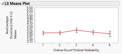
Analysing the LS Means Plot of Ordinal Escort*Ordinal Walkability allows us to visualise that only level 3 seems to have the greatest impact on duration. This level 3 can only be achieved by the combination of Family being the escort, escorting the client in a wheelchair. From this, it is evident that family escorts tend to take a longer moving time with their wheelchair bounded family member.
