Difference between revisions of "REO Project Findings Cluster"
Gtong.2014 (talk | contribs) |
Gtong.2014 (talk | contribs) |
||
| (9 intermediate revisions by the same user not shown) | |||
| Line 38: | Line 38: | ||
| style="padding: 0.25em; font-size: 90%; border-top: 1px solid #cccccc; border-left: 1px solid #cccccc; border-right: 1px solid #cccccc; border-bottom: 1px solid #cccccc; text-align:center; background-color: none; width:30%" | [[REO_Project_Findings_EDA | <font color="#053B6B">Exploratory Data Analysis</font>]] | | style="padding: 0.25em; font-size: 90%; border-top: 1px solid #cccccc; border-left: 1px solid #cccccc; border-right: 1px solid #cccccc; border-bottom: 1px solid #cccccc; text-align:center; background-color: none; width:30%" | [[REO_Project_Findings_EDA | <font color="#053B6B">Exploratory Data Analysis</font>]] | ||
| − | | style="padding: 0.25em; font-size: 90%; border-top: 1px solid #cccccc; border-left: 1px solid #cccccc; border-right: 1px solid #cccccc; border-bottom: 1px solid #cccccc; text-align:center; background-color: #404040; width:30%" | [[REO_Project_Findings_Cluster | <font color="#ffffff"> | + | | style="padding: 0.25em; font-size: 90%; border-top: 1px solid #cccccc; border-left: 1px solid #cccccc; border-right: 1px solid #cccccc; border-bottom: 1px solid #cccccc; text-align:center; background-color: #404040; width:30%" | [[REO_Project_Findings_Cluster | <font color="#ffffff">Clustering Analysis</font>]] |
|} | |} | ||
<br> | <br> | ||
| − | + | ==K-Means Clustering== | |
| − | + | The k-means clustering algorithm is an “iterative algorithm that partitions the observations”. The user input a pre-determined k value, which is the number of partitions. The algorithm begins by first selecting random observations as the starting centroids, then allocate nearby observations to the nearest centroid based on Euclidean distance. A new centroid is calculated from the center of each cluster before each observation is reallocated to the new centroid. The algorithm iterates until either convergence occurs, where there are little to no change in clusters or the maximum number of iteration has occurred. | |
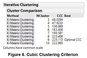
| − | + | <br>The usual process begins with selecting a pre-determined K as the number of clusters. In JMP Pro, the option of selecting a range of clusters was available and the program picks out the most optimal K using the CCC. Based on the CCC, the optimal number of clusters suggested is 9 with the value peaking at 225.113 <br> | |
| − | 3. | + | [[File:REO_fig6.png|300px]]<br> |
| − | The | + | [[File:REO_fig7.png|300px]] |
| − | + | <br>Although the cluster membership appears to be uneven, this is a drastic improvement over the previous iteration. Clusters 3 and 6 are the dominant clusters with their membership exceeding 3000 observations.<br> | |
| − | + | [[File:REO_fig8.png|300px]] | |
| + | <br>The biplot of the clusters indicated several overlaps of the clusters. Clusters 3 and 6 appears to have huge overlaps while there are slight overlaps between 1, 5 and 8. | ||
| + | <br>Such overlaps exist could be due to the issues of high proportion of zero and extreme outliers not being resolved. To resolve the issue of overlapping clusters, the normal mixtures clustering method was used. The optimal K which was developed using the regular K-Means Clustering technique was used as the input K value for normal mixtures. Using JMP Pro, the option to identify outliers and classify them as Cluster 0 was enabled.<br> | ||
| + | [[File:REO_fig9.png|800px]] | ||
| + | <br>Compared to K-Means Analysis, the normal mixtures method was able to resolve the overlapping cluster 3 and 6 by identifying them as one and the same cluster. However, the resulting clusters are not stable as seen by the differing results when the same analysis was conducted thrice. Furthermore, the membership size of the clusters is still largely uneven with overlapping clusters. Therefore, analysis should be done on the output of K-Means Analysis as the results are more stable.<br> | ||
| + | [[File:REO_fig10.png|400px]] | ||
| + | <br>The parallel coordinate plot indicated the various profiles of the segments. The algorithm was able to develop good individual profiles for each of the clusters except for cluster 3 and 6, which appears to exhibit similar characteristics. The previous biplot did suggested that they might be similar due to the overlaps. Despite the slight overlaps for Clusters 1, 5 and 8, the parallel coordinate plot showed that these clusters are different. Therefore, it is recommended that cluster 3 and 6 should be merged to form one cluster. | ||
| + | <br>Aside from clusters 1 and 8, membership of the various clusters appears to be influenced by the type of membership as well due to the dominance of a single class in the clusters.<br> | ||
| + | [[File:REO_fig11.png|300px]] | ||
| + | <br><b>Profiling of Clustering Results</b><br> | ||
| + | [[File:REO_table5.png|600px]] | ||
| + | <br>The clustering analysis was able to develop differentiated profiles. However, it is regrettable that the distribution of the data was not ideal. The datasets are severely skewed due to huge proportions of 0 in all the variables. After filtering out users who have no activity over the past six months, there are approximately only 60% of the initial observations left. Although it is possible to derive stricter criterions to interpret the data and eliminate more skewness, the amount of observations removed would have been unreasonable. For example, if users without at least a session per month are removed, almost half of all observations would have been eliminated. | ||
| + | <br>In addition, the number of observations in each cluster is not balanced. As seen from above, there are 2 dominant group with size of 30.5% and 38.0% while there is sparse membership for two clusters at 0.4% and 1.0%. Cluster size should be generally similar across different clusters so that the effect of segment targeted strategies implemented would be more substantial. | ||
| + | <br>While the k-means clustering algorithm was useful with providing profiles for further business analysis, other types of cluster analysis can be used to segment users more effectively. As such, we would be exploring latent class analysis. | ||
| − | == | + | ==Latent Class Analysis== |
| − | After | + | <b>Discretization of Continuous Variables</b> |
| − | + | <br>To prepare for latent class analysis, the continuous variables need to first be converted into discrete variables. After placing the zeroes into a bin on its own, each continuous variable is then discretized into quartile via the Interactive Binning add-on on JMP. As the fifth bin consists of the extreme outliers as seen below, this would also help to ameliorate the problem of skewness.<br> | |
| − | + | [[File:REO_fig12.png|300px]]<br> | |
| − | [[File: | + | [[File:REO_table6.png|500px]] |
| + | <br><b>Choice of Clusters</b><br> | ||
| + | With the binned scoring classifications, latent class analysis can be performed to determine the clusters. To determine the number of clusters to be used, a selection of 3 to 10 clusters was chosen to determine the best fit of the data into different classes. The Bayesian Information Criteria (BIC) was looked at in order to determine the best model fit. The chosen model is identified by the minimum value of BIC. From the results, the Bayesian information criteria (BIC) was looked at for three to ten clusters and the lowest value was determined to be the model with the best fit. From the table below, we could see that the latent class analysis with six clusters provided the best fit with a BIC value of 121634 and thus, we decided to use the latent class analysis with six clusters and we would be profiling them shortly.<br> | ||
| + | [[File:REO_table7.png|300px]] | ||
| + | <br><b>Discussion on Latent Class Analysis Results</b><br> | ||
| + | [[File:REO_fig13.png|600px]] | ||
| + | <br><b>Interpretation of LCA</b><br> | ||
| + | [[File:REO_table8.png|600px]]<br> | ||
| + | [[File:REO_fig14.png|300px]] | ||
| + | <br> There are paid users in each cluster and that Cluster 3, 5 and 6 have significantly more paid users than free users which is aligned with the interpretation from the table above | ||
| − | === | + | ===Profiling of Clustering Results=== |
| − | + | [[File:REO_table9.png|600px]] | |
| − | [[File: | + | <br><b>Comparison of Observations between K-Means Clusters and LCA Clusters</b> |
| − | <br> | + | Through Mosaic Plot, we can identify the similarities and differences for how the users are categorized into clusters via different techniques.<br> |
| + | [[File:REO_fig15.png|500px]] | ||
| + | <br>The observations clustered using the two different techniques. Based on the mosaic plot, LCA Clusters 1, 2 and 4 exhibited the dominant presence of certain K-Means clusters. As the techniques differ in how the observations are assigned – Euclidean distance vs probability, the differences with the assignment of clusters were expected. | ||
| − | === | + | ===Implications=== |
| − | + | Although both clustering analysis gave reasonably good clusters, the eventual usage of the clusters should be based on the nature of the data and the objective of the research. For REO, the highly skewed distribution of data made it difficult while performing k-means clustering. Hence, the binning process during Latent Class helped to reduce impact of the high proportion of zeroes and extreme outliers. Through creating more even cluster sizes, latent class analysis would help ensure the effect of segment targeted strategies implemented to be more substantial. Therefore, latent class analysis may be more suitable in developing strategies of substantial effect that would reduce attrition rate and hopefully enlarge the potential user base.<br> | |
| − | + | <br>Through the identification of clusters, REO can learn the characteristics of each cluster and develop strategies to increase engagement for each cluster. This debunks REO’s previous assumptions. For example, they would think that most of the paid users are benefiting from the portal but there are significantly high number of subscribers who are either under-performing or have abandoned the platform. They are also not aware of agents who constantly logging in without using other functions on the portal. | |
| − | + | <br><br>Cluster analysis is helpful in identifying customer segments and developing segment specific strategies. In this case, these strategies will increase engagement of users with the portal. Latent class analysis is more effective than k-means clustering in forming distinct clusters of similar sizes. As the profile of agents could change in the future, REO can continually evolve and adapt this process to classify new users. | |
| − | |||
| − | |||
| − | |||
| − | |||
| − | |||
| − | |||
| − | |||
| − | <br> | ||
| − | |||
| − | |||
| − | |||
| − | |||
| − | |||
| − | |||
| − | |||
| − | |||
| − | |||
| − | |||
| − | |||
| − | |||
| − | |||
| − | <br> | ||
| − | |||
| − | |||
| − | |||
| − | |||
| − | |||
| − | |||
| − | |||
| − | |||
| − | |||
| − | |||
| − | |||
| − | |||
| − | |||
| − | |||
| − | |||
| − | |||
| − | |||
| − | |||
| − | |||
| − | |||
Latest revision as of 15:24, 16 April 2018
| Data Preparation | Exploratory Data Analysis | Clustering Analysis |
Contents
K-Means Clustering
The k-means clustering algorithm is an “iterative algorithm that partitions the observations”. The user input a pre-determined k value, which is the number of partitions. The algorithm begins by first selecting random observations as the starting centroids, then allocate nearby observations to the nearest centroid based on Euclidean distance. A new centroid is calculated from the center of each cluster before each observation is reallocated to the new centroid. The algorithm iterates until either convergence occurs, where there are little to no change in clusters or the maximum number of iteration has occurred.
The usual process begins with selecting a pre-determined K as the number of clusters. In JMP Pro, the option of selecting a range of clusters was available and the program picks out the most optimal K using the CCC. Based on the CCC, the optimal number of clusters suggested is 9 with the value peaking at 225.113
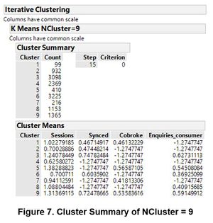
Although the cluster membership appears to be uneven, this is a drastic improvement over the previous iteration. Clusters 3 and 6 are the dominant clusters with their membership exceeding 3000 observations.
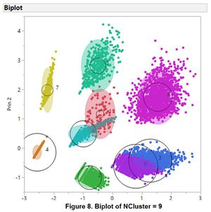
The biplot of the clusters indicated several overlaps of the clusters. Clusters 3 and 6 appears to have huge overlaps while there are slight overlaps between 1, 5 and 8.
Such overlaps exist could be due to the issues of high proportion of zero and extreme outliers not being resolved. To resolve the issue of overlapping clusters, the normal mixtures clustering method was used. The optimal K which was developed using the regular K-Means Clustering technique was used as the input K value for normal mixtures. Using JMP Pro, the option to identify outliers and classify them as Cluster 0 was enabled.
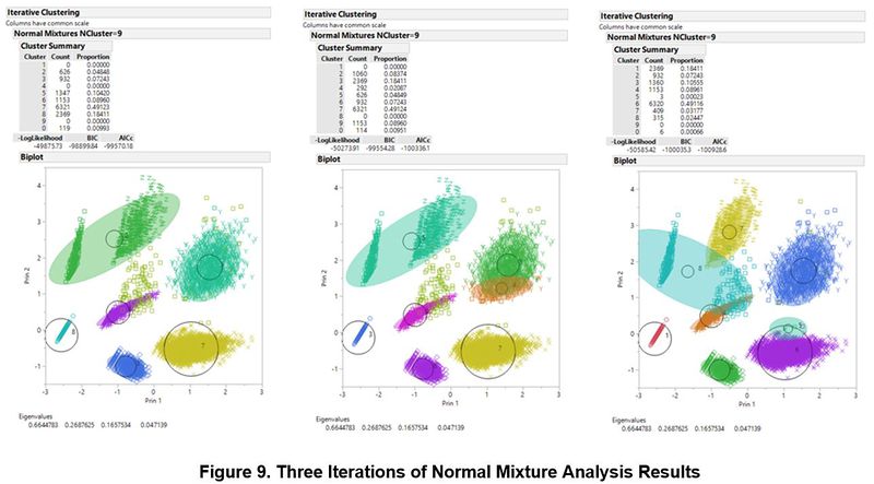
Compared to K-Means Analysis, the normal mixtures method was able to resolve the overlapping cluster 3 and 6 by identifying them as one and the same cluster. However, the resulting clusters are not stable as seen by the differing results when the same analysis was conducted thrice. Furthermore, the membership size of the clusters is still largely uneven with overlapping clusters. Therefore, analysis should be done on the output of K-Means Analysis as the results are more stable.
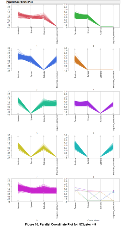
The parallel coordinate plot indicated the various profiles of the segments. The algorithm was able to develop good individual profiles for each of the clusters except for cluster 3 and 6, which appears to exhibit similar characteristics. The previous biplot did suggested that they might be similar due to the overlaps. Despite the slight overlaps for Clusters 1, 5 and 8, the parallel coordinate plot showed that these clusters are different. Therefore, it is recommended that cluster 3 and 6 should be merged to form one cluster.
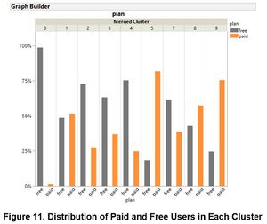
Aside from clusters 1 and 8, membership of the various clusters appears to be influenced by the type of membership as well due to the dominance of a single class in the clusters.
Profiling of Clustering Results
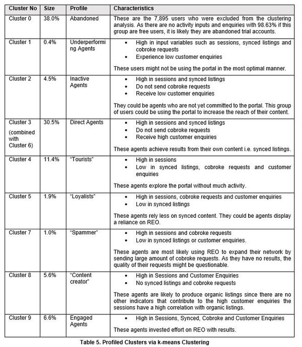
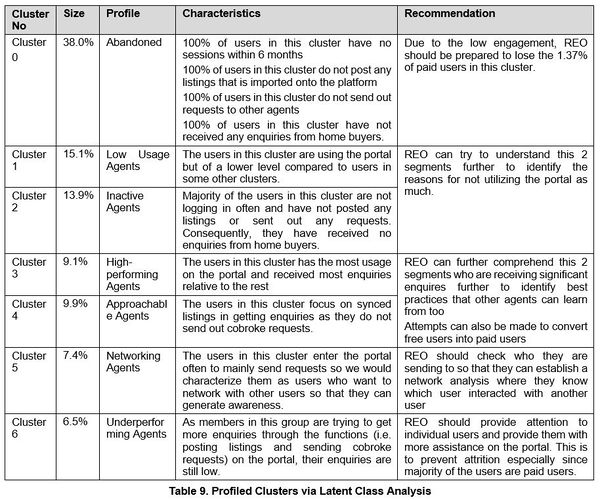
The clustering analysis was able to develop differentiated profiles. However, it is regrettable that the distribution of the data was not ideal. The datasets are severely skewed due to huge proportions of 0 in all the variables. After filtering out users who have no activity over the past six months, there are approximately only 60% of the initial observations left. Although it is possible to derive stricter criterions to interpret the data and eliminate more skewness, the amount of observations removed would have been unreasonable. For example, if users without at least a session per month are removed, almost half of all observations would have been eliminated.
In addition, the number of observations in each cluster is not balanced. As seen from above, there are 2 dominant group with size of 30.5% and 38.0% while there is sparse membership for two clusters at 0.4% and 1.0%. Cluster size should be generally similar across different clusters so that the effect of segment targeted strategies implemented would be more substantial.
While the k-means clustering algorithm was useful with providing profiles for further business analysis, other types of cluster analysis can be used to segment users more effectively. As such, we would be exploring latent class analysis.
Latent Class Analysis
Discretization of Continuous Variables
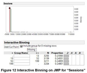
To prepare for latent class analysis, the continuous variables need to first be converted into discrete variables. After placing the zeroes into a bin on its own, each continuous variable is then discretized into quartile via the Interactive Binning add-on on JMP. As the fifth bin consists of the extreme outliers as seen below, this would also help to ameliorate the problem of skewness.

Choice of Clusters
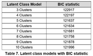
With the binned scoring classifications, latent class analysis can be performed to determine the clusters. To determine the number of clusters to be used, a selection of 3 to 10 clusters was chosen to determine the best fit of the data into different classes. The Bayesian Information Criteria (BIC) was looked at in order to determine the best model fit. The chosen model is identified by the minimum value of BIC. From the results, the Bayesian information criteria (BIC) was looked at for three to ten clusters and the lowest value was determined to be the model with the best fit. From the table below, we could see that the latent class analysis with six clusters provided the best fit with a BIC value of 121634 and thus, we decided to use the latent class analysis with six clusters and we would be profiling them shortly.
Discussion on Latent Class Analysis Results

Interpretation of LCA
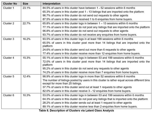
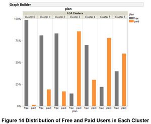
There are paid users in each cluster and that Cluster 3, 5 and 6 have significantly more paid users than free users which is aligned with the interpretation from the table above
Profiling of Clustering Results
Comparison of Observations between K-Means Clusters and LCA Clusters
Through Mosaic Plot, we can identify the similarities and differences for how the users are categorized into clusters via different techniques.
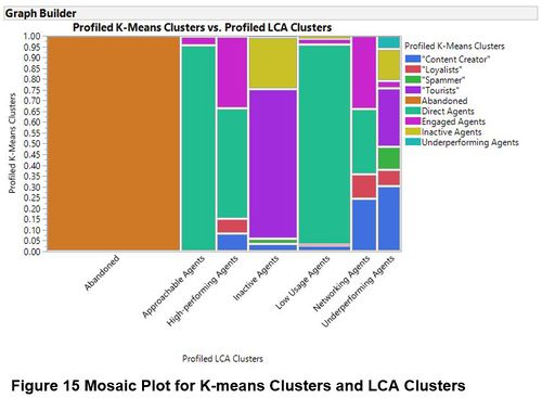
The observations clustered using the two different techniques. Based on the mosaic plot, LCA Clusters 1, 2 and 4 exhibited the dominant presence of certain K-Means clusters. As the techniques differ in how the observations are assigned – Euclidean distance vs probability, the differences with the assignment of clusters were expected.
Implications
Although both clustering analysis gave reasonably good clusters, the eventual usage of the clusters should be based on the nature of the data and the objective of the research. For REO, the highly skewed distribution of data made it difficult while performing k-means clustering. Hence, the binning process during Latent Class helped to reduce impact of the high proportion of zeroes and extreme outliers. Through creating more even cluster sizes, latent class analysis would help ensure the effect of segment targeted strategies implemented to be more substantial. Therefore, latent class analysis may be more suitable in developing strategies of substantial effect that would reduce attrition rate and hopefully enlarge the potential user base.
Through the identification of clusters, REO can learn the characteristics of each cluster and develop strategies to increase engagement for each cluster. This debunks REO’s previous assumptions. For example, they would think that most of the paid users are benefiting from the portal but there are significantly high number of subscribers who are either under-performing or have abandoned the platform. They are also not aware of agents who constantly logging in without using other functions on the portal.
Cluster analysis is helpful in identifying customer segments and developing segment specific strategies. In this case, these strategies will increase engagement of users with the portal. Latent class analysis is more effective than k-means clustering in forming distinct clusters of similar sizes. As the profile of agents could change in the future, REO can continually evolve and adapt this process to classify new users.