Difference between revisions of "AY1718 T2 Group21 Final Findings"
| Line 62: | Line 62: | ||
The outline of the paper is as follows: introduction and motivation behind selecting the client and overall analysis, the literature review – giving a fair characterisation of the literature and research already out there that is relevant to the concepts we’re testing in this paper. Next, the next third part shares the relevant motivation for market basket analysis, and the methodology used implement it, while the fourth section discusses the implementation of MBA and the results we obtained from it. The fifth section mentions our business recommendations according to our understanding of the business and industry, while the final sixth part comprises of a brief conclusion and limitations related to the dataset. | The outline of the paper is as follows: introduction and motivation behind selecting the client and overall analysis, the literature review – giving a fair characterisation of the literature and research already out there that is relevant to the concepts we’re testing in this paper. Next, the next third part shares the relevant motivation for market basket analysis, and the methodology used implement it, while the fourth section discusses the implementation of MBA and the results we obtained from it. The fifth section mentions our business recommendations according to our understanding of the business and industry, while the final sixth part comprises of a brief conclusion and limitations related to the dataset. | ||
<br><br> | <br><br> | ||
| − | The outline of the paper is as follows: first, | + | The outline of the paper is as follows: first, there is an introduction and motivation behind selecting the client and overall analysis. Following this is the literature review - giving a fair characterisation of the literature and research already out there that is relevant to the concepts we’re testing in this paper. The third part then, shares the relevant data structuring for market basket analysis, as well as the methodology used to implement it; which leads onto the next section discussing the implementations of MBA, and the results obtained from it. The paper wraps up with a section on business recommendations according to our understanding of the business and industry, while the final part comprises of a brief conclusion and limitations related to the dataset. |
<br/> | <br/> | ||
<!-- End 1.Introduction --> | <!-- End 1.Introduction --> | ||
| Line 72: | Line 72: | ||
<p style="margin-left: 40px">Market basket analysis (MBA) finds consumer purchase patterns from transactional databases [1]. MBA focuses on discovering buying patterns along thousands or millions of transactions – and here association rules come in handy to identify the correct set and dependencies, to find particular item sets, and relations between purchases between purchased products [2]. | <p style="margin-left: 40px">Market basket analysis (MBA) finds consumer purchase patterns from transactional databases [1]. MBA focuses on discovering buying patterns along thousands or millions of transactions – and here association rules come in handy to identify the correct set and dependencies, to find particular item sets, and relations between purchases between purchased products [2]. | ||
<br> <br> | <br> <br> | ||
| − | Market Basket Analysis uses three keys concepts to come up with association rules: support, confidence and lift. The support of an item is the number of transactions containing that item. Items not meeting the minimum support criteria are excluded from further analysis [6]. The confidence is defined as the conditional probability that a transaction containing the left hand side (LHS) of an association rule, will also contain the right hand side(RHS); whereas lift is a measure of the improvement in the occurrence of the RHS given the LHS: it is the ratio of the conditional probability of the RHS given the LHS, divided by the unconditional probability of the RHS [6]. | + | Market Basket Analysis uses three keys concepts to come up with association rules: support, confidence and lift. The support of an item is the number of transactions containing that item. Items not meeting the minimum support criteria are excluded from further analysis [6]. The confidence is defined as the conditional probability that a transaction containing the left hand side (LHS) of an association rule, will also contain the right hand side(RHS); whereas lift is a measure of the improvement in the occurrence of the RHS given the LHS: it is the ratio of the conditional probability of the RHS given the LHS, divided by the unconditional probability of the RHS [6].</p> |
| − | </p> | ||
[[File:AY1718 T2 Group21 fig1MBA.PNG | 600px | center]] | [[File:AY1718 T2 Group21 fig1MBA.PNG | 600px | center]] | ||
<center><i>Fig. 1: Example of association rules and bundling</i></center> | <center><i>Fig. 1: Example of association rules and bundling</i></center> | ||
<p style="margin-left: 40px"> | <p style="margin-left: 40px"> | ||
As shown in figure 1, given a set of transactions, where each transaction is a set of items, an association rule is an expression X => Y, where X and Y are sets of items. The intuitive meaning of such a rule is that transactions in the database which contain the items in X tend to also contain the items in Y. [9] | As shown in figure 1, given a set of transactions, where each transaction is a set of items, an association rule is an expression X => Y, where X and Y are sets of items. The intuitive meaning of such a rule is that transactions in the database which contain the items in X tend to also contain the items in Y. [9] | ||
| + | <br> | ||
Chapter 16 in the seminal work “Data Mining and Business Analytics with R”, by Johannes Ledolter, discusses how to best structure the data before performing any market basket analysis. As the explanation goes “… (the data) can be arranged in a large matrix of rows and columns. Rows represent the different shoppers (or shopping trips) and columns represent the different products. The entries in the data matrix are the incidences (1 or 0) indicating whether the item in column j of the matrix is purchased by the shopper in row i. The dimensions of the data matrix are usually quite large, with the information on incidences coming from many shoppers (rows) and many different products (columns).” [3] | Chapter 16 in the seminal work “Data Mining and Business Analytics with R”, by Johannes Ledolter, discusses how to best structure the data before performing any market basket analysis. As the explanation goes “… (the data) can be arranged in a large matrix of rows and columns. Rows represent the different shoppers (or shopping trips) and columns represent the different products. The entries in the data matrix are the incidences (1 or 0) indicating whether the item in column j of the matrix is purchased by the shopper in row i. The dimensions of the data matrix are usually quite large, with the information on incidences coming from many shoppers (rows) and many different products (columns).” [3] | ||
</p> | </p> | ||
| Line 94: | Line 94: | ||
<p style="margin-left: 40px"> | <p style="margin-left: 40px"> | ||
We applied the concept of local modelling to our larger dataset of all users, as is described in section 4.8 of “Applied Data Mining for Business and Industry”, [8] where instead of applying the analysis to all possible data points to look for purchasing tendencies and objects visited, we applied to a local subset relevant solely to purchase. Using the entire global sector of all products and all visitors, we utilized this local modelling concept. This was done to keep in line with our true business objective of finding ways to increase the conversion rate based on sales. Looking at visitors’ data and tampering on that account would only pollute our thought process and recommendation ability, as it would describe how to achieve more pageviews and other similar metrics instead. | We applied the concept of local modelling to our larger dataset of all users, as is described in section 4.8 of “Applied Data Mining for Business and Industry”, [8] where instead of applying the analysis to all possible data points to look for purchasing tendencies and objects visited, we applied to a local subset relevant solely to purchase. Using the entire global sector of all products and all visitors, we utilized this local modelling concept. This was done to keep in line with our true business objective of finding ways to increase the conversion rate based on sales. Looking at visitors’ data and tampering on that account would only pollute our thought process and recommendation ability, as it would describe how to achieve more pageviews and other similar metrics instead. | ||
| − | <br><br> | + | <br><br> |
| − | As the book further goes on to say and explain, the concept of Association rules and the data on which association rules are applied are usually in the form of a database of transactions. For each transaction (a row in the database) the database contains the list of items that occur. While in market basket analysis a transaction means a single visit - for which the list of purchases is recorded, in web clickstream analysis a transaction means a web session, for which the list of all visited web pages is recorded [8]. Since each individual may appear more than once in the data set (given how e-commerce tracking works), in the dataset we explore, the paper will be following more along the lines of the web clickstream analysis, where it treats each session (if it differs in origin address and medium) of purchase as one separate transaction. | + | As the book further goes on to say and explain, the concept of Association rules and the data on which association rules are applied are usually in the form of a database of transactions. For each transaction (a row in the database) the database contains the list of items that occur. While in market basket analysis a transaction means a single visit - for which the list of purchases is recorded, in web clickstream analysis a transaction means a web session, for which the list of all visited web pages is recorded [8]. Since each individual may appear more than once in the data set (given how e-commerce tracking works), in the dataset we explore, the paper will be following more along the lines of the web clickstream analysis, where it treats each session (if it differs in origin address and medium) of purchase as one separate transaction.</p> |
| − | </p> | ||
<br> | <br> | ||
<br/> | <br/> | ||
| Line 107: | Line 106: | ||
<div style="background: #a3c665; line-height: 0.3em; font-family:Century Gothic; border-left: #FFFFFF solid 15px;"><div style="border-left: #FFFFFF solid 5px; padding:15px;font-size:15px;"><font color= "#000000"><strong>Explanation of data</strong></font></div></div> | <div style="background: #a3c665; line-height: 0.3em; font-family:Century Gothic; border-left: #FFFFFF solid 15px;"><div style="border-left: #FFFFFF solid 5px; padding:15px;font-size:15px;"><font color= "#000000"><strong>Explanation of data</strong></font></div></div> | ||
<p style="margin-left: 40px"> | <p style="margin-left: 40px"> | ||
| − | + | The data was aggregated over a period of two years, from 8th of March 2016 to 26th of January 2018. During this time, there were a total of 1395 product purchases from 624 customers. The data was exported from Google Analytics and cleaned using Microsoft Excel to be in the right format to import into JMP Pro 13 for further exploration and analysis. | |
<br><br> | <br><br> | ||
| − | Each row of data represents one item purchased by the unique customer, represented by ID. For customers that made multiple purchases from Brainsmith in their lifetime, the rows repeat with the same ID to represent subsequent purchases, as is the necessary structuring to conduct association analysis. The column “ID” is a recoded variable of “ClientID” as there would be data loss of the large integer string (ClientID) when converting files into .csv files that can be imported into JMP Pro 13. | + | Each row of data represents one item purchased by the unique customer, represented by ID. For customers that made multiple purchases from Brainsmith in their lifetime, the rows repeat with the same ID to represent subsequent purchases, as is the necessary structuring to conduct association analysis. The column “ID” is a recoded variable of “ClientID” as there would be data loss of the large integer string (ClientID) when converting files into .csv files that can be imported into JMP Pro 13.</p> |
| − | </p> | ||
[[File:AY1718 T2 Group21 fig3dataset.PNG | 700px | center]] | [[File:AY1718 T2 Group21 fig3dataset.PNG | 700px | center]] | ||
<center><i>Fig. 3: Dataset screenshot</i></center> | <center><i>Fig. 3: Dataset screenshot</i></center> | ||
| Line 127: | Line 125: | ||
<p style="margin-left: 40px"> | <p style="margin-left: 40px"> | ||
As we observe from figure 4, most customers (53%) only purchased 1 item, with the remaining 47% purchasing 2 items or more. The bar representing the number of people that bought just one item is the longest in the histogram. The average number of items that people bought is 2, with a standard deviation of 3. This proves that our data is skewed, and most data points cluster around just purchase quantity values. | As we observe from figure 4, most customers (53%) only purchased 1 item, with the remaining 47% purchasing 2 items or more. The bar representing the number of people that bought just one item is the longest in the histogram. The average number of items that people bought is 2, with a standard deviation of 3. This proves that our data is skewed, and most data points cluster around just purchase quantity values. | ||
| − | + | <br><br> | |
| − | With historical customers’ data showing that there is a 47% occurrence of multiple purchases throughout their shopping experience with Brainsmith, we would be able to observe that Market Basket Analysis could be conducted based on the purchase pattern. This will provide deep insights into the purchase patterns of their users and customers, | + | With historical customers’ data showing that there is a 47% occurrence of multiple purchases throughout their shopping experience with Brainsmith, we would be able to observe that Market Basket Analysis could be conducted based on the purchase pattern. This will provide deep insights into the purchase patterns of their users and customers, and the associations between the products frequently purchased. We next describe the data preparation and methodology we used to conduct the analysis. |
</p> | </p> | ||
<br> | <br> | ||
| Line 187: | Line 185: | ||
<center><i>Table 1: Eight categories of classification</i></center> | <center><i>Table 1: Eight categories of classification</i></center> | ||
<p style="margin-left: 40px"> | <p style="margin-left: 40px"> | ||
| − | Each product was then recoded into their new categories and together with IDs with multiple purchases used for the association analysis as described below. | + | Each product was then recoded into their new categories and together with IDs with multiple purchases used for the association analysis as described below.</p> |
| − | </p> | ||
<br/> | <br/> | ||
<!-- End 3.Data and methoology --> | <!-- End 3.Data and methoology --> | ||
| Line 216: | Line 213: | ||
<div style="background: #a3c665; line-height: 0.3em; font-family:Century Gothic; border-left: #FFFFFF solid 15px;"><div style="border-left: #FFFFFF solid 5px; padding:15px;font-size:15px;"><font color= "#000000"><strong>Frequency and rules</strong></font></div></div> | <div style="background: #a3c665; line-height: 0.3em; font-family:Century Gothic; border-left: #FFFFFF solid 15px;"><div style="border-left: #FFFFFF solid 5px; padding:15px;font-size:15px;"><font color= "#000000"><strong>Frequency and rules</strong></font></div></div> | ||
| + | <br> | ||
| + | <p style="margin-left: 40px">At this point, we ran two association analyses, further complementing the use of local modelling, one with the complete dataset and another without the IDs that only had 1 purchase (i.e. removing 53% of the customers with single purchases, hence removing 23.8% of rows in the dataset). We wanted to investigate how the results of MBA would be different using both datasets. </p> | ||
<br> | <br> | ||
[[File:AY1718 T2 Group21 fig7resultsofassociativeanalysis.PNG| 380px | center]] | [[File:AY1718 T2 Group21 fig7resultsofassociativeanalysis.PNG| 380px | center]] | ||
| − | <center><i>Fig. | + | <center><i>Fig. 7a: Results of associative analysis (entire dataset)</i></center> |
| + | |||
| + | <br> | ||
| + | [[File:AY1718 T2 Group21 fig7bresultsofassociativeanalysis.PNG| 380px | center]] | ||
| + | <center><i>Fig. 7b: Results of associative analysis (without IDs with only 1 purchase)</i></center> | ||
| + | |||
<p style="margin-left: 40px"> | <p style="margin-left: 40px"> | ||
| − | Figure | + | Figure 7a and 7b shows the results of both associative analyses. We can see that there are more rules generated when the analysis was carried out without IDs with 1 purchase. This is due to the increase in support levels for multiple purchases after single purchases were removed. This led to higher confidence levels for item sets resulting in more rules generated. We feel that fig. 7b is more useful for MBA since it is a more representative and specific association analysis for only the multiple purchase transactions.</p> |
| − | + | ||
| + | <p style="margin-left: 40px">To interpret the rules, it indicates that 22% of the customers bought “Plants” and among them, 48% bought “Animals” as well. The lift value is 1.243, indicating a dependency. Also, the rule that has the highest confidence and lift, “Indian” and “People”, shows that 19% of all customers purchased “Indian”, of which 80% bought “People”.</p> | ||
| + | <p style="margin-left: 40px">It is interesting to note that “Animals” and “Packs” which have comparatively high support values of 38% and 15% respectively do not have any associative rules linked to them. Upon closer inspection of the data, we notice that most customers bought products under the “Animals” category together; hence there is no relationship between “Animals” and other product groups. “Packs” are also mostly bought standalone as they already include Quantum Cards, which means customers would be unlikely to buy other products along with it.</p> | ||
</p> | </p> | ||
<br> | <br> | ||
| Line 227: | Line 233: | ||
<div style="background: #a3c665; line-height: 0.3em; font-family:Century Gothic; border-left: #FFFFFF solid 15px;"><div style="border-left: #FFFFFF solid 5px; padding:15px;font-size:15px;"><font color= "#000000"><strong>Singular Value Decomposition</strong></font></div></div> | <div style="background: #a3c665; line-height: 0.3em; font-family:Century Gothic; border-left: #FFFFFF solid 15px;"><div style="border-left: #FFFFFF solid 5px; padding:15px;font-size:15px;"><font color= "#000000"><strong>Singular Value Decomposition</strong></font></div></div> | ||
<p style="margin-left: 40px"> | <p style="margin-left: 40px"> | ||
| − | Singular Value Decomposition (SVD) is a method of analysis to identify items that have an affinity for each other, complementing association analysis. It does so by reducing the SVD of the transaction item matrix into a manageable number of dimensions, hence allowing us to group similar transactions and items. The transaction item matrix is a matrix which each row represents a transaction and each column represents an item, as explained in section 2.1. If the transaction contains an item, the column entry will be one, if not it would be zero | + | Singular Value Decomposition (SVD) is a method of analysis to identify items that have an affinity for each other, complementing association analysis. It does so by reducing the SVD of the transaction item matrix into a manageable number of dimensions, hence allowing us to group similar transactions and items. The transaction item matrix is a matrix which each row represents a transaction and each column represents an item, as explained in section 2.1. If the transaction contains an item, the column entry will be one, if not it would be zero |
<br><br>The SVD approximates the transaction item matrix using three matrixes defined as | <br><br>The SVD approximates the transaction item matrix using three matrixes defined as | ||
<br><br>Transaction Item Matrix ≈ U * S * V’ | <br><br>Transaction Item Matrix ≈ U * S * V’ | ||
| Line 236: | Line 242: | ||
[[File:AY1718 T2 Group21 fig8svdplotoftransactions.PNG| 700px | center]] | [[File:AY1718 T2 Group21 fig8svdplotoftransactions.PNG| 700px | center]] | ||
| − | <center><i>Fig. 8: SVD Plot of transactions </i></center> | + | <center><i>Fig. 8: SVD Plot of transactions for both datasets </i></center> |
<p style="margin-left: 40px"> | <p style="margin-left: 40px"> | ||
| − | In figure 8, the transaction SVD plot on the left represents each transaction as a point, where points visibly grouped together representing similar transactions. From the figure, we can see that there are | + | In figure 8, the transaction SVD plot on the left represents each transaction as a point, where points visibly grouped together representing similar transactions. From the figure, we can see that there are four groups of transactions. The item SVD plot on the right represent each item as a point, plotted against the first two singular vectors in V’. From the same figure, we can see that there are four groups of items with similar functions – a group of Quantum Cards with “World”, “People” and “Indian”, another group of Quantum Cards with “Vehicles”, “Animals” and “Plants”, Wooden Toys and Packs. |
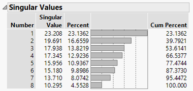
| − | <br><br>The Singular Values Table would then show how much of the spread is explained by the singular vectors, and if the items SVD can clearly represent the dataset. | + | <br><br>The Singular Values Table would then show how much of the spread is explained by the singular vectors, and if the items SVD can clearly represent the dataset. |
</p> | </p> | ||
[[File:AY1718 T2 Group21 fig9singularvaluesofscatterfortransactions.PNG| 380px | center]] | [[File:AY1718 T2 Group21 fig9singularvaluesofscatterfortransactions.PNG| 380px | center]] | ||
<center><i>Fig. 9: Singular values of scatter for transactions</i></center> | <center><i>Fig. 9: Singular values of scatter for transactions</i></center> | ||
| − | <p style="margin-left: 40px">From figure 9, we can see that the first two singular values only explain | + | <p style="margin-left: 40px">From figure 9, we can see that the first two singular values only explain 39.8% of the data spread, meaning additional dimensions may be required to explain the variance. |
</p> | </p> | ||
| Line 251: | Line 257: | ||
<div style="background: #a3c665; line-height: 0.3em; font-family:Century Gothic; border-left: #FFFFFF solid 15px;"><div style="border-left: #FFFFFF solid 5px; padding:15px;font-size:15px;"><font color= "#000000"><strong>Rotated SVD</strong></font></div></div> | <div style="background: #a3c665; line-height: 0.3em; font-family:Century Gothic; border-left: #FFFFFF solid 15px;"><div style="border-left: #FFFFFF solid 5px; padding:15px;font-size:15px;"><font color= "#000000"><strong>Rotated SVD</strong></font></div></div> | ||
<p style="margin-left: 40px"> | <p style="margin-left: 40px"> | ||
| − | We also ran the rotated SVD option which is a varimax rotation on the above SVD of the transaction item matrix. As there are | + | We also ran the rotated SVD option which is a varimax rotation on the above SVD of the transaction item matrix. As there are four groups of transactions, we ran the rotated SVD with four topics. Topics are groups of transactions that are based on primary and secondary item indicators. Every item in each topic has a score that influences its membership in the topic. |
</p> | </p> | ||
[[File:AY1718 T2 Group21 fig10primaryitemswithintopicandscores.PNG| 380px | center]] | [[File:AY1718 T2 Group21 fig10primaryitemswithintopicandscores.PNG| 380px | center]] | ||
<center><i>Fig. 10: Primary items within topic and scores</i></center> | <center><i>Fig. 10: Primary items within topic and scores</i></center> | ||
| − | <p style="margin-left: 40px">The first item listed in each of the topic from figure 10 represent the primary items in the topic. Topic 1 is a group of transactions that contains “People” and | + | <p style="margin-left: 40px">The first item listed in each of the topic from figure 10 represent the primary items in the topic. Topic 1 is a group of transactions that contains “People” and “Indian” but not “Animals”, Topic 2 is a group that contains “Plants” and “Vehicles”, Topic 3 does not contain “Wooden Toys” but contains “World” and Topic 4 contains “Packs” but not “World”. This can further support our association analysis and recommend more specific bundling methods, provided it has sufficiently high support, confidence and lift levels. For our case study, only topic 1 and 2 would be relevant to Brainsmith as it has rules generated to support this analysis. </p> |
| − | |||
| − | |||
<br/> | <br/> | ||
<!-- End 4.Implementation --> | <!-- End 4.Implementation --> | ||
| Line 267: | Line 271: | ||
<div style="background: #a3c665; line-height: 0.3em; font-family:Century Gothic; border-left: #FFFFFF solid 15px;"><div style="border-left: #FFFFFF solid 5px; padding:15px;font-size:15px;"><font color= "#000000"><strong>Method of Bundling</strong></font></div></div> | <div style="background: #a3c665; line-height: 0.3em; font-family:Century Gothic; border-left: #FFFFFF solid 15px;"><div style="border-left: #FFFFFF solid 5px; padding:15px;font-size:15px;"><font color= "#000000"><strong>Method of Bundling</strong></font></div></div> | ||
<p style="margin-left: 40px"> | <p style="margin-left: 40px"> | ||
| − | Based on our market basket analysis, we believe that if Brainsmith decides to bundle products and explore cross-selling, they should bundle products that are in categories that have high confidence values. For instance, they can bundle the products | + | Based on our market basket analysis, we believe that if Brainsmith decides to bundle products and explore cross-selling, they should bundle products that are in categories that have high confidence values. For instance, they can bundle the products “Indian Monuments” and “Organs of the Human Body” together as they are in the “Indian” and “People” categories respectively. By bundling these two products together, there is a likelihood for people to purchase them. |
<br><br>While the company sell bundled Quantum Cards in the “Packs” category, they include products bundled within the same category, limiting cross-selling, and typically include >10 Quantum Cards. Thus, having a smaller product bundled with stronger associative relationship may improve sales. | <br><br>While the company sell bundled Quantum Cards in the “Packs” category, they include products bundled within the same category, limiting cross-selling, and typically include >10 Quantum Cards. Thus, having a smaller product bundled with stronger associative relationship may improve sales. | ||
</p> | </p> | ||
| Line 273: | Line 277: | ||
<div style="background: #a3c665; line-height: 0.3em; font-family:Century Gothic; border-left: #FFFFFF solid 15px;"><div style="border-left: #FFFFFF solid 5px; padding:15px;font-size:15px;"><font color= "#000000"><strong>Product Placement on Website</strong></font></div></div> | <div style="background: #a3c665; line-height: 0.3em; font-family:Century Gothic; border-left: #FFFFFF solid 15px;"><div style="border-left: #FFFFFF solid 5px; padding:15px;font-size:15px;"><font color= "#000000"><strong>Product Placement on Website</strong></font></div></div> | ||
<p style="margin-left: 40px"> | <p style="margin-left: 40px"> | ||
| − | Besides cross-selling, another method that Brainsmith can explore would be to investigate shelf placement of the products. As Brainsmith sells its products online, this would mean that they can explore the order that the products are listed on their catalogue page. Brainsmith can consider placing products from the “People” and “World” categories next to each other on the products sub-page of their website. Also, customers that browse items in one of the categories can have products from the other categories recommended to them in the same page, increasing the likeliness of multiple purchases through association. | + | Besides cross-selling, another method that Brainsmith can explore would be to investigate shelf placement of the products. As Brainsmith sells its products online, this would mean that they can explore the order that the products are listed on their catalogue page. Brainsmith can consider placing products from the “People” and “World” categories next to each other on the products sub-page of their website. Also, customers that browse items in one of the categories can have products from the other categories recommended to them in the same page, increasing the likeliness of multiple purchases through association. |
<br/> | <br/> | ||
<!-- End 5.Recommendations --> | <!-- End 5.Recommendations --> | ||
| Line 286: | Line 290: | ||
<br/> | <br/> | ||
<!-- End 6.Conclusion --> | <!-- End 6.Conclusion --> | ||
| + | |||
| + | <!-- 7. References --> | ||
| + | <div style="background: #688E26; line-height: 0.3em; font-family:Century Gothic; border-left: #FAA613 solid 15px;"><div style="border-left: #FFFFFF solid 5px; padding:15px;font-size:15px;"><font color= "#000000"><strong>REFERENCES</strong></font></div></div> | ||
| + | [1] Linoff G. S., Berry M. J. A. (2011). Data Mining Techniques: For Marketing, Sales, and Customer Relationship Management. John Wiley and Sons, Inc. | ||
| + | <br> | ||
| + | [2] Mauricio, V., Gonzalo, R., Rodrigo, M. (2017). Market basket analysis: Complementing association rules with minimum spanning trees. Expert Systems with Applications. | ||
| + | <br> | ||
| + | [3] Ledolter, J. (2013). Data Mining and Business Analytics with R. John Wiley and Sons, Inc. | ||
| + | <br>[4] Harlam, B. A., Lodish, L. M. (1995). `Modeling Consumers' Choices of Multiple Items. Journal of Marketing Research, 32 (November), 392-403. | ||
| + | <br>[5] Russell, G. J., Petersen, A. (2000). Analysis of Cross Category Dependence in Market Basket Selection. Journal of Retailing; Greenwich Vol. 76, Iss. 3, 367-392. | ||
| + | <br>[6] Qualls, B. (2013) Introduction to Market Basket Analysis. First Analytics, Raleigh, NC. | ||
| + | <br>[7] New Gen App (2017). Market Basket Analysis: Meaning, Benefits and Role of Big Data in MBA. Retrieved from https://www.newgenapps.com/blog/what-is-market-basket-analysis-predicting-customer-purchases-big-data | ||
| + | <br>[8] Giudici, P., Figini, S. (2009). Applied Data Mining for Business and Industry. John Wiley and Sons, Inc. | ||
| + | <br>[9] Agrawal, R., Srikant, R. (1995). Mining Generalized Association Rules. San Jose, California. IBM Research Division. | ||
| + | <br>[10] Senior, J., Springer T., Sherer, Lori. (2016. Reinvigorate Cross-Selling. Retrieved from http://www.bain.com/publications/articles/reinvigorate-cross-selling.aspx | ||
| + | <br> | ||
| + | <br/> | ||
| + | <!-- End References --> | ||
Revision as of 20:25, 15 April 2018
Using Market Basket Analysis and Data-Driven Customer Segmentation and Profiling to Increase e-Commerce Sales of A Children’s Educational e-Commerce Business from India
As the online market rapidly grows today, many businesses turn to the Internet to start their own businesses, setting up e-commerce sites to attract customers from all over the world. Apart from actual sales, owners aim to improve other sales metrics to boost their business, focusing their resources on better marketing materials. With greater outreach, e-commerce sites collect an abundance of data from their visitors.
Working with an online business from India, Brainsmith, the project analyses the significant factors to provide bundling and association rules that could help increase sales. First, exploratory methods were conducted to find customer purchasing behaviour and transactions. Then, Market Basket Analysis was used to analyse the products purchase patterns to find the best bundling packages for Brainsmith. Using two years of website traffic data, the paper focuses on product bundling associations to provide relevant recommendations to boost the website’s sales and conversion rates.
This paper makes use of data analytics techniques to arrive at analysis results, to better optimise processes and sales practices for Brainsmith, a children’s education company based in India that designs and delivers premium educational, learning products and content for early childhood learning and healthy brain development. Data analytics has developed and been implemented over time, and useful results have been observed for a variety of business industries and academic areas. Generically, data analytics is the process of examining data sets to reach conclusions about the information they contain, and increasingly with more specialised tools and software. The company conducts its sales through its website, over the period that we observe their data – and we utilise data analytics to find patterns in the purchase behaviour of their customers according to the data recorded.
The paper takes inspiration from recent literature, that tracks bundling and market baskets in offline product sales, and attempts to further extrapolate it in an e-commerce capacity. While there has been considerable research on the business models involving MBA, this paper hopes to bridge the gap in the internet sales age, and emulates results that have worked in physical stores and attempts to see the results in a virtual environment.
The outline of the paper is as follows: introduction and motivation behind selecting the client and overall analysis, the literature review – giving a fair characterisation of the literature and research already out there that is relevant to the concepts we’re testing in this paper. Next, the next third part shares the relevant motivation for market basket analysis, and the methodology used implement it, while the fourth section discusses the implementation of MBA and the results we obtained from it. The fifth section mentions our business recommendations according to our understanding of the business and industry, while the final sixth part comprises of a brief conclusion and limitations related to the dataset.
The outline of the paper is as follows: first, there is an introduction and motivation behind selecting the client and overall analysis. Following this is the literature review - giving a fair characterisation of the literature and research already out there that is relevant to the concepts we’re testing in this paper. The third part then, shares the relevant data structuring for market basket analysis, as well as the methodology used to implement it; which leads onto the next section discussing the implementations of MBA, and the results obtained from it. The paper wraps up with a section on business recommendations according to our understanding of the business and industry, while the final part comprises of a brief conclusion and limitations related to the dataset.
Market basket analysis (MBA) finds consumer purchase patterns from transactional databases [1]. MBA focuses on discovering buying patterns along thousands or millions of transactions – and here association rules come in handy to identify the correct set and dependencies, to find particular item sets, and relations between purchases between purchased products [2].
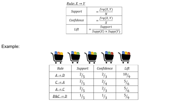
Market Basket Analysis uses three keys concepts to come up with association rules: support, confidence and lift. The support of an item is the number of transactions containing that item. Items not meeting the minimum support criteria are excluded from further analysis [6]. The confidence is defined as the conditional probability that a transaction containing the left hand side (LHS) of an association rule, will also contain the right hand side(RHS); whereas lift is a measure of the improvement in the occurrence of the RHS given the LHS: it is the ratio of the conditional probability of the RHS given the LHS, divided by the unconditional probability of the RHS [6].
As shown in figure 1, given a set of transactions, where each transaction is a set of items, an association rule is an expression X => Y, where X and Y are sets of items. The intuitive meaning of such a rule is that transactions in the database which contain the items in X tend to also contain the items in Y. [9]
Chapter 16 in the seminal work “Data Mining and Business Analytics with R”, by Johannes Ledolter, discusses how to best structure the data before performing any market basket analysis. As the explanation goes “… (the data) can be arranged in a large matrix of rows and columns. Rows represent the different shoppers (or shopping trips) and columns represent the different products. The entries in the data matrix are the incidences (1 or 0) indicating whether the item in column j of the matrix is purchased by the shopper in row i. The dimensions of the data matrix are usually quite large, with the information on incidences coming from many shoppers (rows) and many different products (columns).” [3]
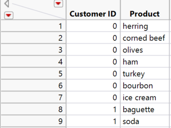
In figure 2, for example, we have rows (i, where i represents from 1 to 9) and columns (j, where j represents CustomerID, Product etc). The incidences in this scenario are mentioned in string form according to which item(s) were purchased by which CustomerID. The software then codes into each Product into 1 or 0 internally (based on whether the corresponding CustomerID has purchased or not) before conducting the MBA.
Market Basket Analysis is a useful technique for companies, and allow to group their products and services in the most optimal manner possible to attract most customers. This could in the future lead to better sales figures, and well influence customer behavior and attract more longevity. By strategically bundling certain products we hope to entice fringe customers (customers that purchase single products in their lifetime) to continue purchasing, and to purchase larger quantities by associating similar products and having pricing strategies conducive to promoting this behaviour. It can also promote cross-selling as a business strategy. Cross-selling is the process through which marketers sell a number of products to their existing customer thus banking on their customer lifetime value. Cross-selling is one of the most used technique to increase revenues and generate ROI from marketing efforts [7]. Market basket analysis helps us identify the products, which the business can look to cross-sell over the lifetime of customers and have a particular customer profiling to send specific email promotions to. For example, Bain & Company’s analysis in 2015-16, in the US telecommunications industry found that up to 60% of customers split their services across multiple providers for mobile phone, landline, TV or Internet services. For one telecoms provider, convincing just 10% of these customers to switch one service from a competitor was worth up to $480 million of incremental annual revenue, thus directly showing the massive potential in sales increase due to cross-sales. [10] This paper will analyse whether this business strategy will be viable based on the forthcoming analysis in this specific case.
We applied the concept of local modelling to our larger dataset of all users, as is described in section 4.8 of “Applied Data Mining for Business and Industry”, [8] where instead of applying the analysis to all possible data points to look for purchasing tendencies and objects visited, we applied to a local subset relevant solely to purchase. Using the entire global sector of all products and all visitors, we utilized this local modelling concept. This was done to keep in line with our true business objective of finding ways to increase the conversion rate based on sales. Looking at visitors’ data and tampering on that account would only pollute our thought process and recommendation ability, as it would describe how to achieve more pageviews and other similar metrics instead.
As the book further goes on to say and explain, the concept of Association rules and the data on which association rules are applied are usually in the form of a database of transactions. For each transaction (a row in the database) the database contains the list of items that occur. While in market basket analysis a transaction means a single visit - for which the list of purchases is recorded, in web clickstream analysis a transaction means a web session, for which the list of all visited web pages is recorded [8]. Since each individual may appear more than once in the data set (given how e-commerce tracking works), in the dataset we explore, the paper will be following more along the lines of the web clickstream analysis, where it treats each session (if it differs in origin address and medium) of purchase as one separate transaction.
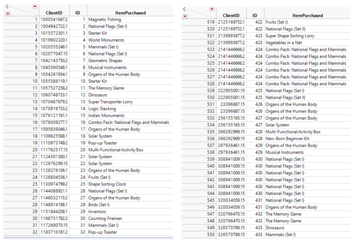
The data was aggregated over a period of two years, from 8th of March 2016 to 26th of January 2018. During this time, there were a total of 1395 product purchases from 624 customers. The data was exported from Google Analytics and cleaned using Microsoft Excel to be in the right format to import into JMP Pro 13 for further exploration and analysis.
Each row of data represents one item purchased by the unique customer, represented by ID. For customers that made multiple purchases from Brainsmith in their lifetime, the rows repeat with the same ID to represent subsequent purchases, as is the necessary structuring to conduct association analysis. The column “ID” is a recoded variable of “ClientID” as there would be data loss of the large integer string (ClientID) when converting files into .csv files that can be imported into JMP Pro 13.
Using this dataset, we proceeded with our exploratory analysis.
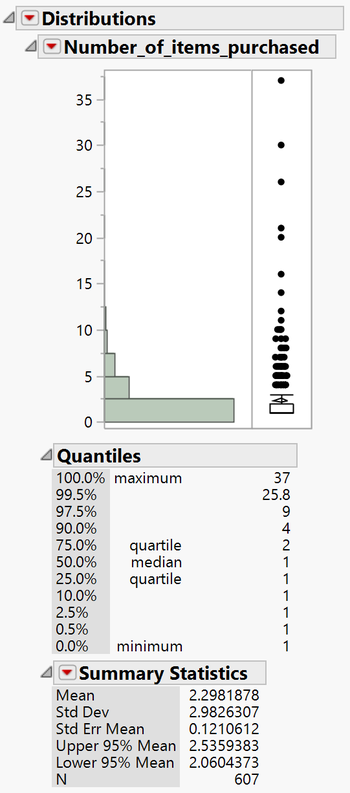
To better understand the data, the centre and spread of the variables involved, we used the following histogram.
As we observe from figure 4, most customers (53%) only purchased 1 item, with the remaining 47% purchasing 2 items or more. The bar representing the number of people that bought just one item is the longest in the histogram. The average number of items that people bought is 2, with a standard deviation of 3. This proves that our data is skewed, and most data points cluster around just purchase quantity values.
With historical customers’ data showing that there is a 47% occurrence of multiple purchases throughout their shopping experience with Brainsmith, we would be able to observe that Market Basket Analysis could be conducted based on the purchase pattern. This will provide deep insights into the purchase patterns of their users and customers, and the associations between the products frequently purchased. We next describe the data preparation and methodology we used to conduct the analysis.
Brainsmith has a total of 113 items in their product catalogue. Upon discussions with the client, eight sub-categories have been used to group the products accordingly to aggregate purchases. These categories have been chosen based on their similarity and substitutability of the products categorized within it - whether products can be easily replaced by others in the same group.
| Category | Description |
|---|---|
| Animals | Quantum Cards related to various individual animals (e.g.: dogs) and categories (e.g.: mammals) |
| Plants | Quantum Cards related to various plants (e.g.: trees) |
| People | Quantum Cards related to important figures (e.g.: inventors) |
| Vehicles | Quantum Cards related to various vehicles (e.g.: construction vehicles) |
| World | Quantum Cards related to the various things around the world (e.g.: national flags) |
| Indian | Quantum Cards related to various important Indian figures |
| Packs | Sets of Quantum Cards |
| Wooden Toys | Wooden Toys sold |
Each product was then recoded into their new categories and together with IDs with multiple purchases used for the association analysis as described below.
After sorting out the individual transactions and sub-categorising the products, an associative analysis was conducted using JMP Pro. This would allow us to identify items that have an affinity for each other and frequently appear together in our transactions, resulting in identifiable relationships between our product categories called association rules, as explored in other literature on this matter. They consist of a conditional item set, of which if present, would predict the item in the consequent item set. Three performance measures determine the strength of association rules – support, confidence, and lift.
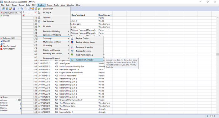
As the three concepts have already been explained and researched into, specifically the importance of these measures are that a high support represents the item set occurring frequently. Confidence is the most important measure as it measures the predictive power of the association rule and a high lift ratio higher than 1 represent that the consequent item set has an affinity to the condition item set. Having established this, moving forward, figure 6 is an example of an association analysis window on JMP Pro. The two variables are selected and assigned to their individual roles. JMP Pro also allows the user to screen the type of rules generated by adjusting the minimum support, confidence and lift for an associative rule. The maximum antecedents control the number of items the condition item set and the maximum rule size controls the number of items that appear in both the condition and consequent item sets. These rules are useful especially for large data sets to obtain more useful results and reduce computational time.
A minimum support of 0.1 implies that the item set appears only 10% of the time, out of all transactions. If product purchase behaviour is more spread out and there is a larger variation in products purchased – i.e. a less observable 20/80 sales pattern – a lower value, such as 0.05, can be considered to generate more rules that would have significant impact on possible bundling. While confidence shows the strength of the rule generated, having a minimum confidence value that is too high may filter significant rules with high support out, leaving highly specific rules for item sets that may have low support. Increasing lift values suggests that the consequent item set occurs more often than expected when the condition item set is present. As a lift value of 1 means that the frequency of the condition and consequent item sets occurring can be expected by chance alone (i.e. not necessarily a relational association between them), the minimum lift value should be higher than 1 to filter rules where the consequent item set has a dependency on the condition item set.
The choice for the values of the maximum antecedents depends on the size of individual transactions. We can expect item sets for rules generated to be larger if the average number of items purchased in a transaction is larger. Since we identified that our average items purchased in a transaction is 2 with a standard deviation of 3 (as explained in section 3.2), we left the maximum antecedents to be 3.
For the purposes of our analysis, the default values were chosen as shown in figure 6.
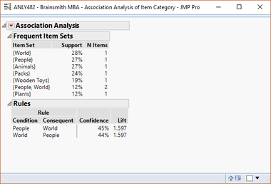
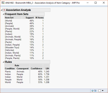
At this point, we ran two association analyses, further complementing the use of local modelling, one with the complete dataset and another without the IDs that only had 1 purchase (i.e. removing 53% of the customers with single purchases, hence removing 23.8% of rows in the dataset). We wanted to investigate how the results of MBA would be different using both datasets.
Figure 7a and 7b shows the results of both associative analyses. We can see that there are more rules generated when the analysis was carried out without IDs with 1 purchase. This is due to the increase in support levels for multiple purchases after single purchases were removed. This led to higher confidence levels for item sets resulting in more rules generated. We feel that fig. 7b is more useful for MBA since it is a more representative and specific association analysis for only the multiple purchase transactions.
To interpret the rules, it indicates that 22% of the customers bought “Plants” and among them, 48% bought “Animals” as well. The lift value is 1.243, indicating a dependency. Also, the rule that has the highest confidence and lift, “Indian” and “People”, shows that 19% of all customers purchased “Indian”, of which 80% bought “People”.
It is interesting to note that “Animals” and “Packs” which have comparatively high support values of 38% and 15% respectively do not have any associative rules linked to them. Upon closer inspection of the data, we notice that most customers bought products under the “Animals” category together; hence there is no relationship between “Animals” and other product groups. “Packs” are also mostly bought standalone as they already include Quantum Cards, which means customers would be unlikely to buy other products along with it.
Singular Value Decomposition (SVD) is a method of analysis to identify items that have an affinity for each other, complementing association analysis. It does so by reducing the SVD of the transaction item matrix into a manageable number of dimensions, hence allowing us to group similar transactions and items. The transaction item matrix is a matrix which each row represents a transaction and each column represents an item, as explained in section 2.1. If the transaction contains an item, the column entry will be one, if not it would be zero
The SVD approximates the transaction item matrix using three matrixes defined as
Transaction Item Matrix ≈ U * S * V’
, where U is the number of rows in the transaction item matrix by the number of singular vectors, S is a diagonal matrix where the entries are the singular values in the SVD and V’ is transpose of vector U.
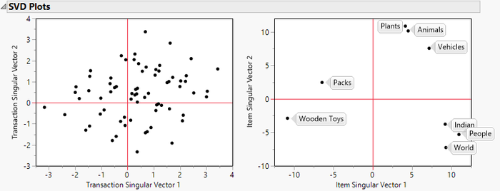
This would help us identify connections among different items that are appearing in the same transactions and also indirect connections where two products that do not appear together in the same transaction, tend to appear together with a third item. These relationships can be plotted onto a scatterplot as shown below.
In figure 8, the transaction SVD plot on the left represents each transaction as a point, where points visibly grouped together representing similar transactions. From the figure, we can see that there are four groups of transactions. The item SVD plot on the right represent each item as a point, plotted against the first two singular vectors in V’. From the same figure, we can see that there are four groups of items with similar functions – a group of Quantum Cards with “World”, “People” and “Indian”, another group of Quantum Cards with “Vehicles”, “Animals” and “Plants”, Wooden Toys and Packs.
The Singular Values Table would then show how much of the spread is explained by the singular vectors, and if the items SVD can clearly represent the dataset.
From figure 9, we can see that the first two singular values only explain 39.8% of the data spread, meaning additional dimensions may be required to explain the variance.
We also ran the rotated SVD option which is a varimax rotation on the above SVD of the transaction item matrix. As there are four groups of transactions, we ran the rotated SVD with four topics. Topics are groups of transactions that are based on primary and secondary item indicators. Every item in each topic has a score that influences its membership in the topic.
The first item listed in each of the topic from figure 10 represent the primary items in the topic. Topic 1 is a group of transactions that contains “People” and “Indian” but not “Animals”, Topic 2 is a group that contains “Plants” and “Vehicles”, Topic 3 does not contain “Wooden Toys” but contains “World” and Topic 4 contains “Packs” but not “World”. This can further support our association analysis and recommend more specific bundling methods, provided it has sufficiently high support, confidence and lift levels. For our case study, only topic 1 and 2 would be relevant to Brainsmith as it has rules generated to support this analysis.
Based on our market basket analysis, we believe that if Brainsmith decides to bundle products and explore cross-selling, they should bundle products that are in categories that have high confidence values. For instance, they can bundle the products “Indian Monuments” and “Organs of the Human Body” together as they are in the “Indian” and “People” categories respectively. By bundling these two products together, there is a likelihood for people to purchase them.
While the company sell bundled Quantum Cards in the “Packs” category, they include products bundled within the same category, limiting cross-selling, and typically include >10 Quantum Cards. Thus, having a smaller product bundled with stronger associative relationship may improve sales.
Besides cross-selling, another method that Brainsmith can explore would be to investigate shelf placement of the products. As Brainsmith sells its products online, this would mean that they can explore the order that the products are listed on their catalogue page. Brainsmith can consider placing products from the “People” and “World” categories next to each other on the products sub-page of their website. Also, customers that browse items in one of the categories can have products from the other categories recommended to them in the same page, increasing the likeliness of multiple purchases through association.
Something we must note, that while researching we observed, was that the purchase data was a little lacking, and quite disparate. This single purchase clients and given the number of purchases that occurred through the website over the past two years, do not provide us enough data to confidently state that our association rules (even within subcategories) are fool-proof. But we believe that this method is robust and can be extended in the future easily as more data is observed.
Through this paper, we attempted to resolve the consistent lack of conversion rate for our client. This resulted in a deep understanding of the e-commerce industry, and the application of traditional retail market analysis techniques to these data sets. What resulted was association rules utilising the past two years of purchase data from past customers.
We hope that recommendations derived from this will provide the company more success and greater direction to bolster sales.
[1] Linoff G. S., Berry M. J. A. (2011). Data Mining Techniques: For Marketing, Sales, and Customer Relationship Management. John Wiley and Sons, Inc.
[2] Mauricio, V., Gonzalo, R., Rodrigo, M. (2017). Market basket analysis: Complementing association rules with minimum spanning trees. Expert Systems with Applications.
[3] Ledolter, J. (2013). Data Mining and Business Analytics with R. John Wiley and Sons, Inc.
[4] Harlam, B. A., Lodish, L. M. (1995). `Modeling Consumers' Choices of Multiple Items. Journal of Marketing Research, 32 (November), 392-403.
[5] Russell, G. J., Petersen, A. (2000). Analysis of Cross Category Dependence in Market Basket Selection. Journal of Retailing; Greenwich Vol. 76, Iss. 3, 367-392.
[6] Qualls, B. (2013) Introduction to Market Basket Analysis. First Analytics, Raleigh, NC.
[7] New Gen App (2017). Market Basket Analysis: Meaning, Benefits and Role of Big Data in MBA. Retrieved from https://www.newgenapps.com/blog/what-is-market-basket-analysis-predicting-customer-purchases-big-data
[8] Giudici, P., Figini, S. (2009). Applied Data Mining for Business and Industry. John Wiley and Sons, Inc.
[9] Agrawal, R., Srikant, R. (1995). Mining Generalized Association Rules. San Jose, California. IBM Research Division.
[10] Senior, J., Springer T., Sherer, Lori. (2016. Reinvigorate Cross-Selling. Retrieved from http://www.bain.com/publications/articles/reinvigorate-cross-selling.aspx

