Difference between revisions of "APA Feature Engineering"
m (color change) |
(change f.eng's navi. bar) |
||
| (20 intermediate revisions by 2 users not shown) | |||
| Line 5: | Line 5: | ||
<font face="Century Gothic"> | <font face="Century Gothic"> | ||
{| style="background-color:#FFFFFF; color:#66ffcc padding: 5px 0 0 0;" width="100%" cellspacing="0" cellpadding="0" valign="top" border="0" | | {| style="background-color:#FFFFFF; color:#66ffcc padding: 5px 0 0 0;" width="100%" cellspacing="0" cellpadding="0" valign="top" border="0" | | ||
| − | | style="padding:0.3em; font-family:Helvetica; font-size:120%; border-bottom:2px solid #66ffcc; border-top:2px solid #66ffcc; border-left:2px solid #66ffcc; background:#66ffcc; text-align:center;" width=" | + | | style="padding:0.3em; font-family:Helvetica; font-size:120%; border-bottom:2px solid #66ffcc; border-top:2px solid #66ffcc; border-left:2px solid #66ffcc; background:#66ffcc; text-align:center;" width="8%" | |
[https://wiki.smu.edu.sg/ANLY482/ANLY482_AY2016-17_T2_Group17 <font face ="Century Gothic" color="#000000"><strong>HOME</strong></font>] | [https://wiki.smu.edu.sg/ANLY482/ANLY482_AY2016-17_T2_Group17 <font face ="Century Gothic" color="#000000"><strong>HOME</strong></font>] | ||
| style="border-bottom:2px solid #66ffcc; border-top:2px solid #66ffcc; background:#66ffcc;" width="1%" | | | style="border-bottom:2px solid #66ffcc; border-top:2px solid #66ffcc; background:#66ffcc;" width="1%" | | ||
| − | | style="padding:0.3em; font-family:Helvetica; font-size:120%; border-bottom:2px solid #66ffcc; border-top:2px solid #66ffcc; background:#66ffcc; text-align:center;" width=" | + | | style="padding:0.3em; font-family:Helvetica; font-size:120%; border-bottom:2px solid #66ffcc; border-top:2px solid #66ffcc; background:#66ffcc; text-align:center;" width="15%" | |
[[APA_Project Overview|<font face ="Century Gothic" color="#000000"><strong> PROJECT OVERVIEW</strong></font>]] | [[APA_Project Overview|<font face ="Century Gothic" color="#000000"><strong> PROJECT OVERVIEW</strong></font>]] | ||
| style="border-bottom:2px solid #66ffcc; border-top:2px solid #66ffcc; background:#66ffcc;" width="1%" | | | style="border-bottom:2px solid #66ffcc; border-top:2px solid #66ffcc; background:#66ffcc;" width="1%" | | ||
| − | | style="padding:0.3em; font-family:Helvetica; font-size:120%; border-bottom:2px solid #66ffcc; border-top:2px solid #66ffcc; background:#66ffcc; text-align:center;" width=" | + | | style="padding:0.3em; font-family:Helvetica; font-size:120%; border-bottom:2px solid #66ffcc; border-top:2px solid #66ffcc; background:#66ffcc; text-align:center;" width="12%" | |
| − | [[APA_Final_Progress|<font face ="Century Gothic" color="#000000"><strong> | + | [[APA_Final_Progress|<font face ="Century Gothic" color="#000000"><strong> METHODOLOGY</strong></font>]] |
| style="border-bottom:2px solid #66ffcc; border-top:2px solid #66ffcc; background:#66ffcc;" width="1%" | | | style="border-bottom:2px solid #66ffcc; border-top:2px solid #66ffcc; background:#66ffcc;" width="1%" | | ||
| − | | style="padding:0.3em; font-family:Helvetica; font-size:120%; border-bottom:2px solid #66ffcc; border-top:2px solid #66ffcc; background:# | + | | style="padding:0.3em; font-family:Helvetica; font-size:120%; border-bottom:2px solid #66ffcc; border-top:2px solid #66ffcc; background:#ffffff; text-align:center;" width="18%" | |
| − | [[ | + | [[APA_Feature Engineering|<font face ="Century Gothic" color="#66ffcc"><strong> FEATURE ENGINEERING</strong></font>]] |
| style="border-bottom:2px solid #66ffcc; border-top:2px solid #66ffcc; background:#66ffcc;" width="1%" | | | style="border-bottom:2px solid #66ffcc; border-top:2px solid #66ffcc; background:#66ffcc;" width="1%" | | ||
| − | | style="padding:0.3em; font-family:Helvetica; font-size:120%; border-bottom:2px solid #66ffcc; border-top:2px solid #66ffcc; background:#66ffcc; text-align:center;" width=" | + | | style="padding:0.3em; font-family:Helvetica; font-size:120%; border-bottom:4px solid #66ffcc; border-top:4px solid #66ffcc; background:#66ffcc; text-align:center;" width="18%" | |
| + | [[APA_Project_Management|<font face ="Century Gothic" color="#000000"><strong>CLASSIFICATION MODELLING </strong></font>]] | ||
| + | | style="border-bottom:2px solid #66ffcc; border-top:2px solid #66ffcc; background:#66ffcc;" width="1%" | | ||
| + | | style="padding:0.3em; font-family:Helvetica; font-size:120%; border-bottom:2px solid #66ffcc; border-top:2px solid #66ffcc; background:#66ffcc; text-align:center;" width="12%" | | ||
[[APA_Documentation|<font face ="Century Gothic" color="#000000"><strong> DOCUMENTATION</strong></font>]] | [[APA_Documentation|<font face ="Century Gothic" color="#000000"><strong> DOCUMENTATION</strong></font>]] | ||
| style="border-bottom:2px solid #66ffcc; border-top:2px solid #66ffcc; background:#66ffcc;" width="1%" | | | style="border-bottom:2px solid #66ffcc; border-top:2px solid #66ffcc; background:#66ffcc;" width="1%" | | ||
| − | | style="padding:0.3em; font-family:Helvetica; font-size:120%; border-bottom:2px solid # | + | | style="padding:0.3em; font-family:Helvetica; font-size:120%; border-bottom:2px solid #45c198; border-top:2px solid #45c198; background:#66ffcc; text-align:center;" width="17%" | |
| − | [[ | + | [[ANLY482_AY2016-17_Term_2|<font face ="Century Gothic" color="#000000"><strong>OTHER PROJECTS</strong></font>]] |
| style="border-bottom:2px solid #66ffcc; border-top:2px solid #66ffcc; background:#66ffcc;" width="1%" | | | style="border-bottom:2px solid #66ffcc; border-top:2px solid #66ffcc; background:#66ffcc;" width="1%" | | ||
| − | | style=" | + | | style="font-family:Helvetica; font-size:120%; border-bottom:4px solid #45c198; border-top:4px solid #45c198; background:#66ffcc; text-align:center;" width="20%" | |
| − | |||
| − | |||
| − | |||
| − | |||
|} | |} | ||
<br> | <br> | ||
| Line 34: | Line 33: | ||
<P> | <P> | ||
'''Subject Line weightage:''' | '''Subject Line weightage:''' | ||
| − | |||
| − | |||
| − | |||
| − | |||
| − | |||
| − | |||
| − | |||
| − | |||
| − | |||
| − | |||
| − | |||
| − | |||
<br> | <br> | ||
| + | This feature is used to show the quality of information exchanged between any two employees. Since, there is no access to the body of the emails, this feature is based on the subject lines of emails exchanged between employees. A higher weightage is given to a subject line which contains more work-related terms. These work-related terms are generated using text mining. The average weightage is then taken for all emails exchanged between each unique pair of employees. This feature helps in quantitatively analyzing subject lines’ importance based on their term weightages.<br><br> | ||
| + | This feature is derived in the following steps. Firstly, SAS Enterprise Miner is used to conduct text mining, where the first step is to import data using the ‘File Import’ node. This node is then connected to the ‘Text Parsing’ node where certain configurations must be done to adjust the results of text mining as required. The text parsing node should then be connected to the ‘Text Filter’ node, where configurations for the type of term weighting and thresholds can be set. Below is a diagram of the process flow as will be seen in SAS Enterprise Miner. <br><br> | ||
| + | [[File:TMprocess.jpg|400px]] | ||
| + | <br><br> | ||
| + | The main aspects to take note of for text parsing are: | ||
| + | <ol><li>Ignoring the types of entities:<br> | ||
| + | Depending on the context of the analysis, certain entities must be ignored to give relevant results. For instance, if a dataset has a high frequency of currency occurrence, then currencies must be removed from the analysis because it is not relevant. Some of the entities removed were ‘Address’, ‘Currency’, ‘Date’, ‘Percent’, ‘Phone’ and ‘Time’. </li> | ||
| + | <li>Ignoring the types of attributes:<br> | ||
| + | Certain attributes that are unimportant to the analysis, such as numbers and punctuations in the case of this study, can be ignored. Number and punctuations are unlikely to provide any insights when mining short texts such as email subject lines as in the case of this study. </li> | ||
| + | <li>Ignoring the parts of speech:<br> | ||
| + | Parts of speech are often meaningless words that have a high occurrence in text documents. Such words are likely to skew results and thus it is good to remove them to keep the focus on more important and meaningful words. Some of the parts of speech that were removed were ‘aux’, ‘conj’, ‘det’, ‘num’ and ‘part’.</li> | ||
| + | <li>Including the stop list:<br> | ||
| + | A stop list is a list of stop words which are words that have little value in determining the importance of the document. In this study, a text mining analysis is run with the default list of stop words initially. Upon eyeballing through the text mining results, selected terms from the results are added to the stop list as they are of little value. For example, some of the terms added to the stop list were “18th”, “7am” and “Automatic reply”. The objective of the stop list for this study is to retain as many business-related words only. </li></ol> | ||
| + | <br><br> | ||
| + | The main aspects to take note of for text filter are: | ||
| + | <ol><li>Determining the method of term weighting:<br> | ||
| + | The term weighting method for short documents such as email subject lines used in this study is ‘Inverse Document Frequency (IDF) Log’ (after referring to the paper by Mika Timonen (2013)). IDF is a measure of how rare or common a term occurs across all documents. The minimum Number of Documents is taken as 30. </li> | ||
| + | <li>Handling synonyms:<br> | ||
| + | The final step under text filter is to treat words such as ‘run’ and ‘running’ as synonyms to prevent the text mining process from treating them as two different words with different meanings and hence possibly diluting the importance of the word.</li></ol> | ||
| + | <br><br> | ||
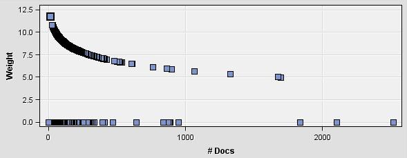
| + | After the configurations are complete, the process can be run, finally giving a set of words with their term frequency values, frequency of occurrence, number of documents that each respective word appeared in and more. Due to the way IDF calculates term weights, the results show that terms with high frequencies, and with occurrences in a high number of documents have low weightages as shown below. | ||
| + | <br><br> | ||
| + | [[File:idf.jpg|600px]] | ||
| + | <br><br> | ||
| + | To reverse this, a new term weightage is calculated by taking an inverse of IDF weights from the original results: <br><br> | ||
| + | Final Term Weightage= 1/(IDF Weight)<br><br> | ||
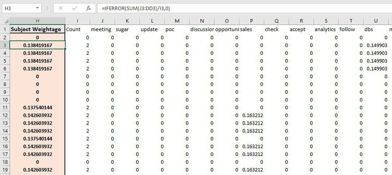
| + | Based on these weights, the top 100 business related words are selected as the list of weighted words with which to calculate the email subject line weightages. Let’s call this list the subject-line-weight-list (SLWL). For each email exchange tuple in the data, a subject line weightage is calculated by checking of an instance of the terms in the SLWL in the email’s subject line. If the term exists, then it is aggregated. Finally, the sum of all weightages of all the terms that occur in the subject line are divided by the count of terms from SLWL (shown in ‘Count’ column in excel sheet) present in the subject line. This finally gives an average weight. <br><br> | ||
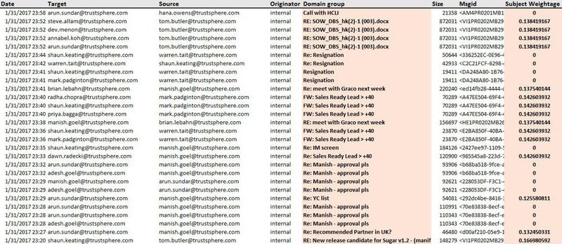
| + | The subject line weights are aggregated using Microsoft Excel as shown below. Each row represents each subject line from the email data. For that row, if the term is present, the cell value is replaced with the term’s weight, otherwise with 0. The ‘Subject Weightage’ column then sums across all columns in that row and averages it out by the count of terms from SLWL. The final results of the calculation are as presented in Figure 17, based on the terms from SLWL ().<br><br> | ||
| + | [[File:slwl.jpg|800px]] | ||
| + | <br><br> | ||
| + | The final results of the calculation are as presented below, based on the terms from SLWL ().<br><br> | ||
| + | [[File:TMresults.jpg|800px]] | ||
| + | <br><br> | ||
| + | As shown before, the subject lines have been assigned a weightage based on the words they contain. This weightage is used to calculate “Subject Line Weightage” using the following formula: | ||
| + | <br><br> | ||
| + | <i>Average (Subject weightage of all emails exchanged between A and B)</i> | ||
| + | <br><br> | ||
| + | The email data with the subject weights is imported into phpmyadmin and SQL is used to apply the above formula onto the data to get proper output. The SQL statement used to apply this formula is given below: | ||
| + | <br><br> | ||
| + | <font face="Courier New">Select least(‘Target’, ‘Source’) as employee1, greatest (‘Target’, ‘Source’) as employee2, avg(‘Subject Weightage’) as subjectweight from subject group by least(‘Target’, ‘Source’) , greatest(‘Target’, ‘Source’);</font> | ||
| + | <br><br> | ||
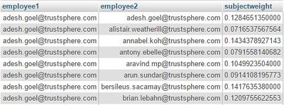
| + | In the above SQL statement, ‘Source’ is the sender of the email while ‘Target’ is the receiver of the email. The variable ‘Subject Weightage’ corresponds to the weight of the subjects of the emails. A part of the results is shown in the table below: | ||
| + | <br><br> | ||
| + | [[File:SLWresults.JPG|400px]] | ||
| + | <br><br> | ||
'''Email Exchange Ratio:'''<br> | '''Email Exchange Ratio:'''<br> | ||
| − | This | + | This feature is used to show the frequency of information exchanged between any two employees. It is used to check the number of emails exchanged between two employees to show how much they interact, collaborate, and share information. The formula used for this feature is: |
| − | + | <br><br> | |
| − | <div style="text-align: center;"> | + | <div style="border:1px solid rgb(85,198,225); -moz-border-radius:15px;width:250px;padding:10px;text-align: center;"> |
| − | [[Image:EmailExchangeRatioFormula.PNG|200px]] | + | [[Image:EmailExchangeRatioFormula.PNG|200px]] <br> |
| − | + | 𝑁𝑎𝑏: Number of emails exchanged between A and B <br> | |
| − | </div> | + | 𝑁𝑎: Number of emails sent by A <br> |
| − | < | + | 𝑁𝑏:Number of emails sent by B |
| − | <br> | + | </div><br> |
| + | The email data is imported into phpmyadmin and SQL is used to apply the above formula onto the data to get proper output. The SQL statement used to apply this formula is given below:<br><br> | ||
| + | <font face="Courier New">select t1.employee1, t1.employee2, (t1.total/(IFNULL(t2.total,0) + IFNULL(t3.total,0) - t1.total)) as EmailExchangedRatio from | ||
| + | (select least(`Remote`,`Local`) as employee1, greatest(`Remote`,`Local`) as employee2, count(*) as total from midterm group by least(`Remote`,`Local`), greatest(`Remote`,`Local`)) as t1 | ||
| + | |||
| + | left join (select `Local` as employee, count(*) as total from midterm group by `Local`) as t2 on t2.employee = t1.employee1 | ||
| + | |||
| + | left join (select `Local` as employee, count(*) as total from midterm group by `Local`) as t3 on t3.employee = t1.employee2;</font> | ||
| + | <br><br> | ||
| + | In this SQL statement, ‘Local’ is the sender of the email while ‘Remote’ is the receiver of the email. A part of the results is shown in the table below: | ||
| + | <br><br> | ||
| + | [[Image:EmailExchangeRatioResults.jpg|400px]] | ||
| + | <br><br> | ||
'''Average Email Exchange Size:'''<br> | '''Average Email Exchange Size:'''<br> | ||
| − | This | + | This feature is used to show the quantity of information exchanged between any two employees. Assuming that a larger email size shows larger amount of information exchange, the following formula is used to calculate the average email exchange size: |
| − | < | + | <br><br> |
| − | + | <i>Average (Size of all emails exchangedbetween A and B) </i> | |
| − | + | <br><br> | |
| − | [[Image:EmailexSizeResults.png|400px]]< | + | The email data is imported into phpmyadmin and SQL is used to apply the above formula onto the data to get proper output. The SQL statement used to apply this formula is given below. |
| − | <br> | + | <br><br> |
| + | <font face="Courier New">select least(`Remote`,`Local`) as employee1, greatest(`Remote`,`Local`) as employee2, avg(size) from midterm group by least(`Remote`,`Local`), greatest(`Remote`,`Local`);</font> | ||
| + | <br><br> | ||
| + | In this SQL statement, ‘Local’ is the sender of the email while ‘Remote’ is the receiver of the email. The variable ‘size’ corresponds to the size of the email. A part of the results is shown in the table below: | ||
| + | <br><br> | ||
| + | [[Image:EmailexSizeResults.png|400px]] | ||
| + | <br><br> | ||
'''Email Chain Ratio:'''<br> | '''Email Chain Ratio:'''<br> | ||
| − | This | + | This feature is used to show the variety of information exchanged between any two employees. The assumption that unique conversations taking place in emails show variety of information being shared was made. Thus, number of emails with unique subject lines shows number of different conversations taking place between employees through email data. To capture this, the following formula is used: |
| − | + | <br><br> | |
| − | <div style="text-align: center;"> | + | <div style="border:1px solid rgb(85,198,225); -moz-border-radius:15px;width:250px;padding:10px;text-align: center;"> |
| − | [[ | + | [[File:ECRformula.jpg|200px]] <br> |
| − | + | 𝑁𝑎𝑏: Number of emails exchanged between A and B <br> | |
| − | [[ | + | 𝑁𝑢: Number of emails exchanged between A and B with unique subject lines<br> |
| − | <br> | + | </div><br><br> |
| + | The email data is imported into phpmyadmin and SQL is used to apply the above formula onto the data to get proper output. The SQL statement used to apply this formula is given below: | ||
| + | <br><br> | ||
| + | <font face="Courier New">SELECT t1.employee1, t1.employee2, (t1.uniqueEmails/t1.total) as ratio from | ||
| + | (SELECT least(`Remote`,`Local`) as employee1, greatest(`Remote`,`Local`) as employee2, count(*) as total, | ||
| + | count( distinct `Domain group`) as uniqueEmails FROM midterm group by least(`Remote`,`Local`), greatest(`Remote`,`Local`)) as t1;</font> | ||
| + | <br><br> | ||
| + | In this SQL statement, ‘Local’ is the sender of the email while ‘Remote’ is the receiver of the email. The variable “Domain Group” corresponds to the subject line of the email. A part of the results is shown in the table below: | ||
| + | <br><br> | ||
| + | [[File:ECRresults.jpg|400px]] | ||
| + | <br><br> | ||
'''Rate of exchange of emails:'''<br> | '''Rate of exchange of emails:'''<br> | ||
| − | This | + | This feature is used to show the regularity of information exchanged between any two employees. It is used to show how regularly employees interact with one another. The following formula is used: |
| − | <div style="text-align: center;"> | + | <br><br> |
| − | [[ | + | <div style="border:1px solid rgb(85,198,225); -moz-border-radius:15px;width:250px;padding:10px;text-align: center;"> |
| − | + | [[File:RATEformula.jpg|200px]] <br> | |
| − | [[Image:RateOfExchangeResults.PNG|400px]] | + | 𝑁𝑎𝑏: Number of emails exchanged between A and B <br> |
| + | c: Number of weeks<br> | ||
| + | </div><br> | ||
| + | The email data is imported into phpmyadmin and SQL is used to apply the above formula onto the data to get proper output. The SQL statement used to apply this formula is given below. | ||
| + | <br><br> | ||
| + | <font face="Courier New">(select least(`Remote`,`Local`) as employee1, greatest(`Remote`,`Local`) as employee2, (count(*)/10) as total from midterm group by least(`Remote`,`Local`), greatest(`Remote`,`Local`))</font> | ||
| + | <br><br> | ||
| + | In this SQL statement, ‘Local’ is the sender of the email while ‘Remote’ is the receiver of the email. Number of emails exchanged between employees is divided by 10 because our data spans over 10 weeks. A part of the results is shown in the table below: | ||
| + | <br><br> | ||
| + | [[Image:RateOfExchangeResults.PNG|400px]] | ||
<br> | <br> | ||
Latest revision as of 19:40, 23 April 2017
Subject Line weightage:
This feature is used to show the quality of information exchanged between any two employees. Since, there is no access to the body of the emails, this feature is based on the subject lines of emails exchanged between employees. A higher weightage is given to a subject line which contains more work-related terms. These work-related terms are generated using text mining. The average weightage is then taken for all emails exchanged between each unique pair of employees. This feature helps in quantitatively analyzing subject lines’ importance based on their term weightages.
This feature is derived in the following steps. Firstly, SAS Enterprise Miner is used to conduct text mining, where the first step is to import data using the ‘File Import’ node. This node is then connected to the ‘Text Parsing’ node where certain configurations must be done to adjust the results of text mining as required. The text parsing node should then be connected to the ‘Text Filter’ node, where configurations for the type of term weighting and thresholds can be set. Below is a diagram of the process flow as will be seen in SAS Enterprise Miner.

The main aspects to take note of for text parsing are:
- Ignoring the types of entities:
Depending on the context of the analysis, certain entities must be ignored to give relevant results. For instance, if a dataset has a high frequency of currency occurrence, then currencies must be removed from the analysis because it is not relevant. Some of the entities removed were ‘Address’, ‘Currency’, ‘Date’, ‘Percent’, ‘Phone’ and ‘Time’. - Ignoring the types of attributes:
Certain attributes that are unimportant to the analysis, such as numbers and punctuations in the case of this study, can be ignored. Number and punctuations are unlikely to provide any insights when mining short texts such as email subject lines as in the case of this study. - Ignoring the parts of speech:
Parts of speech are often meaningless words that have a high occurrence in text documents. Such words are likely to skew results and thus it is good to remove them to keep the focus on more important and meaningful words. Some of the parts of speech that were removed were ‘aux’, ‘conj’, ‘det’, ‘num’ and ‘part’. - Including the stop list:
A stop list is a list of stop words which are words that have little value in determining the importance of the document. In this study, a text mining analysis is run with the default list of stop words initially. Upon eyeballing through the text mining results, selected terms from the results are added to the stop list as they are of little value. For example, some of the terms added to the stop list were “18th”, “7am” and “Automatic reply”. The objective of the stop list for this study is to retain as many business-related words only.
The main aspects to take note of for text filter are:
- Determining the method of term weighting:
The term weighting method for short documents such as email subject lines used in this study is ‘Inverse Document Frequency (IDF) Log’ (after referring to the paper by Mika Timonen (2013)). IDF is a measure of how rare or common a term occurs across all documents. The minimum Number of Documents is taken as 30. - Handling synonyms:
The final step under text filter is to treat words such as ‘run’ and ‘running’ as synonyms to prevent the text mining process from treating them as two different words with different meanings and hence possibly diluting the importance of the word.
After the configurations are complete, the process can be run, finally giving a set of words with their term frequency values, frequency of occurrence, number of documents that each respective word appeared in and more. Due to the way IDF calculates term weights, the results show that terms with high frequencies, and with occurrences in a high number of documents have low weightages as shown below.
To reverse this, a new term weightage is calculated by taking an inverse of IDF weights from the original results:
Final Term Weightage= 1/(IDF Weight)
Based on these weights, the top 100 business related words are selected as the list of weighted words with which to calculate the email subject line weightages. Let’s call this list the subject-line-weight-list (SLWL). For each email exchange tuple in the data, a subject line weightage is calculated by checking of an instance of the terms in the SLWL in the email’s subject line. If the term exists, then it is aggregated. Finally, the sum of all weightages of all the terms that occur in the subject line are divided by the count of terms from SLWL (shown in ‘Count’ column in excel sheet) present in the subject line. This finally gives an average weight.
The subject line weights are aggregated using Microsoft Excel as shown below. Each row represents each subject line from the email data. For that row, if the term is present, the cell value is replaced with the term’s weight, otherwise with 0. The ‘Subject Weightage’ column then sums across all columns in that row and averages it out by the count of terms from SLWL. The final results of the calculation are as presented in Figure 17, based on the terms from SLWL ().
The final results of the calculation are as presented below, based on the terms from SLWL ().
As shown before, the subject lines have been assigned a weightage based on the words they contain. This weightage is used to calculate “Subject Line Weightage” using the following formula:
Average (Subject weightage of all emails exchanged between A and B)
The email data with the subject weights is imported into phpmyadmin and SQL is used to apply the above formula onto the data to get proper output. The SQL statement used to apply this formula is given below:
Select least(‘Target’, ‘Source’) as employee1, greatest (‘Target’, ‘Source’) as employee2, avg(‘Subject Weightage’) as subjectweight from subject group by least(‘Target’, ‘Source’) , greatest(‘Target’, ‘Source’);
In the above SQL statement, ‘Source’ is the sender of the email while ‘Target’ is the receiver of the email. The variable ‘Subject Weightage’ corresponds to the weight of the subjects of the emails. A part of the results is shown in the table below:
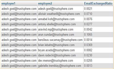
Email Exchange Ratio:
This feature is used to show the frequency of information exchanged between any two employees. It is used to check the number of emails exchanged between two employees to show how much they interact, collaborate, and share information. The formula used for this feature is:

𝑁𝑎𝑏: Number of emails exchanged between A and B
𝑁𝑎: Number of emails sent by A
𝑁𝑏:Number of emails sent by B
The email data is imported into phpmyadmin and SQL is used to apply the above formula onto the data to get proper output. The SQL statement used to apply this formula is given below:
select t1.employee1, t1.employee2, (t1.total/(IFNULL(t2.total,0) + IFNULL(t3.total,0) - t1.total)) as EmailExchangedRatio from
(select least(`Remote`,`Local`) as employee1, greatest(`Remote`,`Local`) as employee2, count(*) as total from midterm group by least(`Remote`,`Local`), greatest(`Remote`,`Local`)) as t1
left join (select `Local` as employee, count(*) as total from midterm group by `Local`) as t2 on t2.employee = t1.employee1
left join (select `Local` as employee, count(*) as total from midterm group by `Local`) as t3 on t3.employee = t1.employee2;
In this SQL statement, ‘Local’ is the sender of the email while ‘Remote’ is the receiver of the email. A part of the results is shown in the table below:
Average Email Exchange Size:
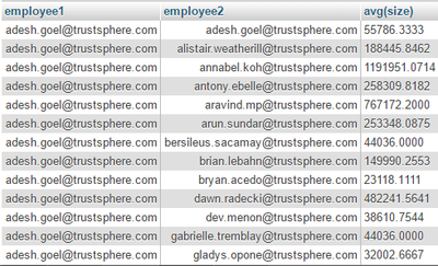
This feature is used to show the quantity of information exchanged between any two employees. Assuming that a larger email size shows larger amount of information exchange, the following formula is used to calculate the average email exchange size:
Average (Size of all emails exchangedbetween A and B)
The email data is imported into phpmyadmin and SQL is used to apply the above formula onto the data to get proper output. The SQL statement used to apply this formula is given below.
select least(`Remote`,`Local`) as employee1, greatest(`Remote`,`Local`) as employee2, avg(size) from midterm group by least(`Remote`,`Local`), greatest(`Remote`,`Local`);
In this SQL statement, ‘Local’ is the sender of the email while ‘Remote’ is the receiver of the email. The variable ‘size’ corresponds to the size of the email. A part of the results is shown in the table below:
Email Chain Ratio:
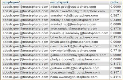
This feature is used to show the variety of information exchanged between any two employees. The assumption that unique conversations taking place in emails show variety of information being shared was made. Thus, number of emails with unique subject lines shows number of different conversations taking place between employees through email data. To capture this, the following formula is used:

𝑁𝑎𝑏: Number of emails exchanged between A and B
𝑁𝑢: Number of emails exchanged between A and B with unique subject lines
The email data is imported into phpmyadmin and SQL is used to apply the above formula onto the data to get proper output. The SQL statement used to apply this formula is given below:
SELECT t1.employee1, t1.employee2, (t1.uniqueEmails/t1.total) as ratio from
(SELECT least(`Remote`,`Local`) as employee1, greatest(`Remote`,`Local`) as employee2, count(*) as total,
count( distinct `Domain group`) as uniqueEmails FROM midterm group by least(`Remote`,`Local`), greatest(`Remote`,`Local`)) as t1;
In this SQL statement, ‘Local’ is the sender of the email while ‘Remote’ is the receiver of the email. The variable “Domain Group” corresponds to the subject line of the email. A part of the results is shown in the table below:
Rate of exchange of emails:
This feature is used to show the regularity of information exchanged between any two employees. It is used to show how regularly employees interact with one another. The following formula is used:
The email data is imported into phpmyadmin and SQL is used to apply the above formula onto the data to get proper output. The SQL statement used to apply this formula is given below.
(select least(`Remote`,`Local`) as employee1, greatest(`Remote`,`Local`) as employee2, (count(*)/10) as total from midterm group by least(`Remote`,`Local`), greatest(`Remote`,`Local`))
In this SQL statement, ‘Local’ is the sender of the email while ‘Remote’ is the receiver of the email. Number of emails exchanged between employees is divided by 10 because our data spans over 10 weeks. A part of the results is shown in the table below:


