Difference between revisions of "Analysis and Findings as of Finals"
(Undo revision 11827 by Dina.heng.2013 (talk)) |
|||
| (22 intermediate revisions by 2 users not shown) | |||
| Line 69: | Line 69: | ||
The list below shows the 4 different models identified: | The list below shows the 4 different models identified: | ||
| − | # Regression Model | + | # Multiple Regression Model |
# Decision Tree Model | # Decision Tree Model | ||
# Boosted Tree Model | # Boosted Tree Model | ||
# Bootstrap Forest Model | # Bootstrap Forest Model | ||
| − | Out of the 4 models above, all the models other than Regression Model are classified as eager learners. Since there is no provision of train and test datasets, our team will need to craft our own datasets with the following proportions as shown below: | + | Out of the 4 models above, all the models other than Multiple Regression Model are classified as eager learners. Since there is no provision of train and test datasets, our team will need to craft our own datasets with the following proportions as shown below: |
| − | {| class="wikitable" | + | <center> |
| + | {| class="wikitable" | style="text-align: center" | ||
|- | |- | ||
! Dataset !! Proportion | ! Dataset !! Proportion | ||
| Line 87: | Line 88: | ||
|- | |- | ||
|} | |} | ||
| + | </center> | ||
| − | * Regression Model | + | * '''Multiple Regression Model''' |
| − | The Regression Model allows us to explore and understand the relationship between a dependent variable (in our case, this is the tickets sold) and one or more independent variables (in this case, this is the derived variables in the previous subsection). | + | The Multiple Regression Model allows us to explore and understand the relationship between a dependent variable (in our case, this is the tickets sold) and one or more independent variables (in this case, this is the derived variables in the previous subsection). |
Prior to the calibration of the model, our team has decided to log-transform the number of tickets sold to assume a normal distribution, so that our model will not be dominated by extreme values. | Prior to the calibration of the model, our team has decided to log-transform the number of tickets sold to assume a normal distribution, so that our model will not be dominated by extreme values. | ||
| − | [[File:RegressionModel-LogTransformTicketsSold.JPG| | + | [[File:RegressionModel-LogTransformTicketsSold.JPG|500px|center|Comparison of Before and After Log-Transform Tickets Sold Distribution]] |
| − | + | As from the model calibrated based on the derived variables, our team managed to achieve a decent result as shown in the table below. | |
| + | <center> | ||
| + | {| class="wikitable" | style="text-align: center" | ||
| + | |- | ||
| + | ! Dataset !! R-Square !! RMSE | ||
| + | |- | ||
| + | | Train Data || 0.747 || 0.213 | ||
| + | |- | ||
| + | | Validation Data || 0.742 || 0.214 | ||
| + | |- | ||
| + | | Test Data || 0.746 || 0.211 | ||
| + | |- | ||
| + | |} | ||
| + | </center> | ||
| + | |||
| + | As from the results generated from the model, it shows a decent R-Square value at approximately 0.74, and comparing the R-Square and RMSE value across all the 3 datasets, it shows that there are very signs of over-fitting and under-fitting. | ||
| + | |||
| + | [[File:RegressionModel-EffectsSummary-1.JPG|600px|center|Effect Summary]] | ||
| + | |||
| + | And looking at the Effects Summary of the model, as shown above, it further shows that almost all of the variables played a significant amount of influence, except for the "Day" variable. Next, our team performed a step-wise regression analysis, which is an effective approach in selecting variables to be used in the model and this can help us to improve our model performance. | ||
| + | |||
| + | The following images document the process of performing stepwise-regression analysis. | ||
| + | |||
| + | [[File:RegressionModel-Stepwise-1.JPG|400px|center|Adding Variables]] | ||
| + | |||
| + | |||
| + | [[File:RegressionModel-Stepwise-2.JPG|400px|center|Configuring Stepwise Regression Control]] | ||
| + | |||
| + | |||
| + | [[File:RegressionModel-Stepwise-3.JPG|400px|center|Variable selected from Stepwise Regression]] | ||
| + | |||
| + | |||
| + | In the current estimates image, it shows the result which the Stepwise Multiple Regression Model attempted to create and select a hierarchy from within the different variables. And this selection behaviour seemed to repeat itself throughout other variables as well, and thus, our team concluded that even though the R-Square value did not drop much as compared to our initial Multiple Regression Model, the Regression approach may not after all be a suitable approach as there are too much categorical effects within the model. Thus, we will be focusing our attention on the tree-based model to combat such issues. | ||
| + | |||
| + | |||
| + | |||
| + | * '''Decision Tree Model''' | ||
| + | |||
| + | The Decision Tree Model consists of multiple splits in a single tree, where each of the splits can have a decision or possible consequences, and the splitting of variables is determined by entropy value. Contrary to the log-transformation used in the Multiple Regression Model, the Decision Tree Model does not require any log-transformation. | ||
| + | |||
| + | |||
| + | The table below shows the results generated from the Decision Tree Model: | ||
| + | |||
| + | <center> | ||
| + | {| class="wikitable" | style="text-align: center" | ||
| + | |- | ||
| + | ! Dataset !! R-Square !! RMSE | ||
| + | |- | ||
| + | | Train Data || 0.813 || 4691.75 | ||
| + | |- | ||
| + | | Validation Data || 0.775 || 5094.41 | ||
| + | |- | ||
| + | | Test Data || 0.783 || 5003.52 | ||
| + | |- | ||
| + | |} | ||
| + | </center> | ||
| + | |||
| + | |||
| + | As from the result, it can be seen that the R-Square value is slightly higher across all datasets as compared to the Multiple Regression Model, however it can observed that this specific model is showing signs of over-fitting, as the RMSE is higher for test datasets than train datasets. | ||
| + | |||
| + | |||
| + | |||
| + | * '''Boosted Tree Model''' | ||
| + | |||
| + | As from the Decision Tree Model, we would like to also use a more sophisticated decision tree model, and observe if the results would improve or not. | ||
| + | |||
| + | In Boosted Tree Model, it works similar to a Decision Tree Model, however each of the sub-trees is generated from residuals from the previous trees. Finally, the final tree will then combine all the sub-trees to form the final tree. The diagram below shows the concept of how Boosted Tree is being generated. | ||
| + | |||
| + | [[File:BoostedTree-Concept.JPG|500px|center|Concept of Boosted Tree Model]] | ||
| + | |||
| + | The table below shows the results generated from the Boosted Tree Model: | ||
| + | |||
| + | <center> | ||
| + | {| class="wikitable" | style="text-align: center" | ||
| + | |- | ||
| + | ! Dataset !! R-Square !! RMSE | ||
| + | |- | ||
| + | | Train Data || 0.864 || 4000.27 | ||
| + | |- | ||
| + | | Validation Data || 0.810 || 4673.70 | ||
| + | |- | ||
| + | | Test Data || 0.814 || 4625.73 | ||
| + | |- | ||
| + | |} | ||
| + | </center> | ||
| + | |||
| + | As observed from the results, it can be observed that the R-Square value are overall higher, as compared to the Decision Tree Model. The RMSE is also lower as compared to the previous model, which indicates the accuracy of the model. However, at a closer look between all 3 datasets, it can be seen that there is a greater amount of overfitting, where the test error alot higher than the train error. | ||
| + | |||
| + | |||
| + | |||
| + | * '''Bootstrap Forest Model''' | ||
| + | |||
| + | Similarly, our team also tested out the Bootstrap Forest Model. The Bootstrap Forest Model generates multiple trees, where each of these trees is being generated based on random sample. It will then combine the trees generated from random sample, and tries to get the best result by averaging the score of each tree. The diagram below shows the concept of how Bootstrap Forest is being generated. | ||
| + | |||
| + | [[File:BootstrapForest-Concept.JPG|500px|center|Concept of Boosted Tree Model]] | ||
| + | |||
| + | The table below shows the results generated from the Bootstrap Forest Model: | ||
| + | |||
| + | <center> | ||
| + | {| class="wikitable" align=center | style="text-align: center" | ||
| + | |- | ||
| + | ! Dataset !! R-Square !! RMSE | ||
| + | |- | ||
| + | | Train Data || 0.818 || 4629.6 | ||
| + | |- | ||
| + | | Validation Data || 0.771 || 5135.6 | ||
| + | |- | ||
| + | | Test Data || 0.802 || 4774.6 | ||
| + | |- | ||
| + | |} | ||
| + | </center> | ||
| + | |||
| + | From the results, it can be observed that the overall RMSE across all 3 datasets are all higher than those in the Boosted Tree Model. However, upon comparison of the results from the 3 datasets, it can be seen that the train and test errors are both closer, and thus shows signs of less over-fitting. | ||
| + | |||
| + | |||
| + | |||
| + | * '''Model Comparison''' | ||
| + | |||
| + | <center> | ||
| + | {| class="wikitable" align=center | style="text-align: center" | ||
| + | |- | ||
| + | ! Models !! R-Square !! RMSE || AAE | ||
| + | |- | ||
| + | | Decision Tree || 0.796 || 4878.4 || 3075.4 | ||
| + | |- | ||
| + | | Boosted Tree || 0.838 || 4339.7 || 2738.3 | ||
| + | |- | ||
| + | | Boostrap Forest || 0.803 || 4785.1 || 2982.2 | ||
| + | |- | ||
| + | |} | ||
| + | </center> | ||
| − | * | + | *Legend: |
| + | **AAE - Average Absolute Error. | ||
| − | + | With reference to the above table, the comparison of models have shown that Boosted Tree Model has shown the best result. However, it must be noted that to the client that the Boosted Tree is also the model which has the strongest signs out of overfitting, with its test errors higher than the train errors. | |
| + | The graph below shows the accuracy of the Boosted Tree Model, with the actual tickets sold vs the predicted tickets sold. | ||
| + | [[File:Model_ActualvsPredicted.png|800px|center|Concept of Boosted Tree Model]] | ||
</div> | </div> | ||
Latest revision as of 13:22, 9 February 2017
| Mid-Term | Finals |
|---|
As from the Data Exploration phase up till Mid-Terms, our team has realized that there are numerous factors that will possibly each of the different events. Therefore, our team has decided to put forward the factors, as shown in the table below, which will be used to assist us in building predictive models to explain the variations in the demands or tickets sold for each event.
| No. | Factors | Description |
|---|---|---|
| 1 | Concurrent Events | Our team is hypothesizing that the events, which started at the same time period will make people buy less tickets. There might be a possibility that if there are more concurrent events ongoing, the demand may be split across the concurrent events. |
| 2 | Day of Week | The day of the week will also potentially affect the demands for each event, as events which are held in the weekdays may be attract less customers than events held over the weekends. |
| 3 | Event Name | As from our Exploratory Analysis, we realized that each of the events perform differently, and there are a multitude of factors which affects its variations in demands. |
| 4 | Time Period | Our team chose to divide 24-hours in a single day to 3-hours time block (e.g., 12AM to 2:59AM as Early Midnight & 3AM to 5:59AM as Late Midnight), as different customers might prefer events due to their lifestyle. |
| 5 | Month | The month factor is important as there might be a possibility that certain months, such as the holiday or festive season, which will potentially attract more customers to buy tickets for the different events. |
With all the identified factors, our team prepared the data to be in a suitable data structure to be fed into our predictive model in the Model Calibration and Validation phase.
In this phase, our team has identified 4 different models, and the aim of this phase is to calibrate the identified models based on the above derived variables and evaluate its performance through the Root Mean Square Error (RMSE).
The list below shows the 4 different models identified:
- Multiple Regression Model
- Decision Tree Model
- Boosted Tree Model
- Bootstrap Forest Model
Out of the 4 models above, all the models other than Multiple Regression Model are classified as eager learners. Since there is no provision of train and test datasets, our team will need to craft our own datasets with the following proportions as shown below:
| Dataset | Proportion |
|---|---|
| Train Data | 50% |
| Validation Data | 20% |
| Test Data | 30% |
- Multiple Regression Model
The Multiple Regression Model allows us to explore and understand the relationship between a dependent variable (in our case, this is the tickets sold) and one or more independent variables (in this case, this is the derived variables in the previous subsection).
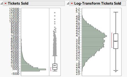
Prior to the calibration of the model, our team has decided to log-transform the number of tickets sold to assume a normal distribution, so that our model will not be dominated by extreme values.
As from the model calibrated based on the derived variables, our team managed to achieve a decent result as shown in the table below.
| Dataset | R-Square | RMSE |
|---|---|---|
| Train Data | 0.747 | 0.213 |
| Validation Data | 0.742 | 0.214 |
| Test Data | 0.746 | 0.211 |
As from the results generated from the model, it shows a decent R-Square value at approximately 0.74, and comparing the R-Square and RMSE value across all the 3 datasets, it shows that there are very signs of over-fitting and under-fitting.
And looking at the Effects Summary of the model, as shown above, it further shows that almost all of the variables played a significant amount of influence, except for the "Day" variable. Next, our team performed a step-wise regression analysis, which is an effective approach in selecting variables to be used in the model and this can help us to improve our model performance.
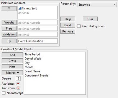
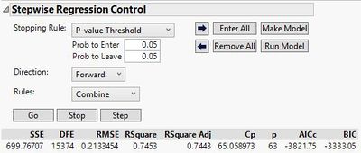
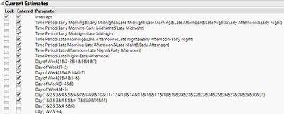
The following images document the process of performing stepwise-regression analysis.
In the current estimates image, it shows the result which the Stepwise Multiple Regression Model attempted to create and select a hierarchy from within the different variables. And this selection behaviour seemed to repeat itself throughout other variables as well, and thus, our team concluded that even though the R-Square value did not drop much as compared to our initial Multiple Regression Model, the Regression approach may not after all be a suitable approach as there are too much categorical effects within the model. Thus, we will be focusing our attention on the tree-based model to combat such issues.
- Decision Tree Model
The Decision Tree Model consists of multiple splits in a single tree, where each of the splits can have a decision or possible consequences, and the splitting of variables is determined by entropy value. Contrary to the log-transformation used in the Multiple Regression Model, the Decision Tree Model does not require any log-transformation.
The table below shows the results generated from the Decision Tree Model:
| Dataset | R-Square | RMSE |
|---|---|---|
| Train Data | 0.813 | 4691.75 |
| Validation Data | 0.775 | 5094.41 |
| Test Data | 0.783 | 5003.52 |
As from the result, it can be seen that the R-Square value is slightly higher across all datasets as compared to the Multiple Regression Model, however it can observed that this specific model is showing signs of over-fitting, as the RMSE is higher for test datasets than train datasets.
- Boosted Tree Model
As from the Decision Tree Model, we would like to also use a more sophisticated decision tree model, and observe if the results would improve or not.
In Boosted Tree Model, it works similar to a Decision Tree Model, however each of the sub-trees is generated from residuals from the previous trees. Finally, the final tree will then combine all the sub-trees to form the final tree. The diagram below shows the concept of how Boosted Tree is being generated.
The table below shows the results generated from the Boosted Tree Model:
| Dataset | R-Square | RMSE |
|---|---|---|
| Train Data | 0.864 | 4000.27 |
| Validation Data | 0.810 | 4673.70 |
| Test Data | 0.814 | 4625.73 |
As observed from the results, it can be observed that the R-Square value are overall higher, as compared to the Decision Tree Model. The RMSE is also lower as compared to the previous model, which indicates the accuracy of the model. However, at a closer look between all 3 datasets, it can be seen that there is a greater amount of overfitting, where the test error alot higher than the train error.
- Bootstrap Forest Model
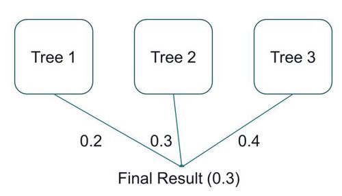
Similarly, our team also tested out the Bootstrap Forest Model. The Bootstrap Forest Model generates multiple trees, where each of these trees is being generated based on random sample. It will then combine the trees generated from random sample, and tries to get the best result by averaging the score of each tree. The diagram below shows the concept of how Bootstrap Forest is being generated.
The table below shows the results generated from the Bootstrap Forest Model:
| Dataset | R-Square | RMSE |
|---|---|---|
| Train Data | 0.818 | 4629.6 |
| Validation Data | 0.771 | 5135.6 |
| Test Data | 0.802 | 4774.6 |
From the results, it can be observed that the overall RMSE across all 3 datasets are all higher than those in the Boosted Tree Model. However, upon comparison of the results from the 3 datasets, it can be seen that the train and test errors are both closer, and thus shows signs of less over-fitting.
- Model Comparison
| Models | R-Square | RMSE | AAE |
|---|---|---|---|
| Decision Tree | 0.796 | 4878.4 | 3075.4 |
| Boosted Tree | 0.838 | 4339.7 | 2738.3 |
| Boostrap Forest | 0.803 | 4785.1 | 2982.2 |
- Legend:
- AAE - Average Absolute Error.
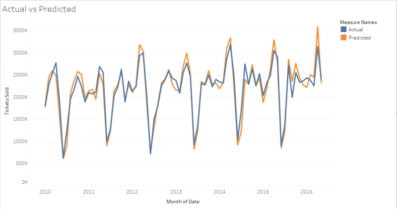
With reference to the above table, the comparison of models have shown that Boosted Tree Model has shown the best result. However, it must be noted that to the client that the Boosted Tree is also the model which has the strongest signs out of overfitting, with its test errors higher than the train errors.
The graph below shows the accuracy of the Boosted Tree Model, with the actual tickets sold vs the predicted tickets sold.
