Difference between revisions of "ANLY482 AY2016-17 T1 Group1: PROJECT FINDINGS/Post"
| (One intermediate revision by the same user not shown) | |||
| Line 78: | Line 78: | ||
<div><font face="Roboto"> | <div><font face="Roboto"> | ||
'''Problem Definition''' | '''Problem Definition''' | ||
| + | |||
In measuring the performance of SGAG’s Facebook posts, the reach of the post which is defined as the total number of users who have seen a particular post is commonly used among the social media content creators. Nevertheless, it is challenging for them to determine the various components that may possibly affect this KPI with merely human judgement. Thus, an attempt to utilize the multiple linear regression analysis in examining these factors influencing the KPI will be discussed in the following section. | In measuring the performance of SGAG’s Facebook posts, the reach of the post which is defined as the total number of users who have seen a particular post is commonly used among the social media content creators. Nevertheless, it is challenging for them to determine the various components that may possibly affect this KPI with merely human judgement. Thus, an attempt to utilize the multiple linear regression analysis in examining these factors influencing the KPI will be discussed in the following section. | ||
'''Analysis Methodology''' | '''Analysis Methodology''' | ||
| + | |||
As mentioned previously, Multiple Linear Regressions can be developed using the Fit Model platform of JMP Pro by selecting the response variable (Y axis) which is Post’s reach (Lifetime Organic Post Reach) and the explanatory variables (X axis) which comprises of various continuous variables such as Main Engagement and Negative Feedbacks. Categorical variables will be added to the model once multicollinearity is eliminated from the model. | As mentioned previously, Multiple Linear Regressions can be developed using the Fit Model platform of JMP Pro by selecting the response variable (Y axis) which is Post’s reach (Lifetime Organic Post Reach) and the explanatory variables (X axis) which comprises of various continuous variables such as Main Engagement and Negative Feedbacks. Categorical variables will be added to the model once multicollinearity is eliminated from the model. | ||
[[File:ANLY482_Group1_Figure2.png|400px|center]] | [[File:ANLY482_Group1_Figure2.png|400px|center]] | ||
| − | + | [[File:ANLY482_Group1_Figure3.png|300px|center]] | |
| − | [[File:ANLY482_Group1_Figure3.png| | ||
| − | |||
As seen from Figure 3, 97% of variability of the response variable can be explained by the explanatory variables. High R-Square indicates high accuracy of the model. Nonetheless, multicollinearity will need to firstly be examined in order to attain the true factors affecting the KPI. | As seen from Figure 3, 97% of variability of the response variable can be explained by the explanatory variables. High R-Square indicates high accuracy of the model. Nonetheless, multicollinearity will need to firstly be examined in order to attain the true factors affecting the KPI. | ||
[[File:ANLY482_Group1_Figure4.png|400px|center]] | [[File:ANLY482_Group1_Figure4.png|400px|center]] | ||
| − | |||
From Figure 4 above, the highlighted columns such as Lifetime Engaged Users and Hide Clicks per thousand user indicate variables with VIF of larger than 8. These variables will be re-selected through the use of variables clustering analysis to eliminate the multicollinearity. | From Figure 4 above, the highlighted columns such as Lifetime Engaged Users and Hide Clicks per thousand user indicate variables with VIF of larger than 8. These variables will be re-selected through the use of variables clustering analysis to eliminate the multicollinearity. | ||
[[File:ANLY482_Group1_Figure5.png|400px|center]] | [[File:ANLY482_Group1_Figure5.png|400px|center]] | ||
| − | |||
[[File:ANLY482_Group1_Figure6.png|400px|center]] | [[File:ANLY482_Group1_Figure6.png|400px|center]] | ||
| − | |||
| + | As shown in Figure 6, there were two clusters formed and the representative variables are Main Engagement and No of negative feedback per thousand users. Hence, other variables will be removed from the model and the model will be re-run and further evaluated. | ||
| + | |||
| + | [[File:ANLY482_Group1_Figure7.png|400px|center]] | ||
| + | |||
| + | From Figure 7, the remaining independent variables are those with VIF < 8. After eliminating multicollinearity from the model, we will now attempt to filter insignificant factors from this model. As explained previously, variables with p-value (Prob>|t|) of larger than 0.05 are considered as insignificant and the highlighted factor (Post Message Length) have a p-value of 0.18. Therefore, will be removed from the model to improve the true accuracy of the model. Afterwhich, categorical variables such as type and public holiday will also be included to the model. | ||
| + | |||
| + | '''Results''' | ||
| + | [[File:ANLY482_Group1_Figure9.png|300px|center]] | ||
| + | [[File:ANLY482_Group1_Figure10.png|400px|center]] | ||
| + | |||
| + | The final model and its reports can be seen from Figure 9 and 10. In this model, 89.5% of the variability of the response variable (Post Reach) can be explained by the various independent variables (Main Engagement, Number of Negative Feedbacks per thousand user, Hide All Clicks per thousand user, Unlike Page per thousand user, Type). The VIF of the explanatory variables are lesser than 8, indicating no multicollinearity exists and p-value of all variables are lesser than 0.0001 indicating strong it is a strong model. | ||
| + | |||
| + | Equation representing the relationship between the dependent variable and the independent variables can be written as such: | ||
| + | |||
| + | '''Post Reach''' = '''6.60''' (intercept) + '''0.27''' ( Log[Main Engagement] ) + '''0.05''' ( Log[No of negative feedback per thousand user] ) - '''0.17''' ( Log[Hide All Clicks per thousand user] ) - '''0.58''' ( Log[Unlike Page per thousand user] )+ Match( Type )("Link" → '''-0.05''', "Photo" → '''- 0.16''', "Video" → '''0.21''') | ||
| + | |||
| + | [[File:ANLY482_Group1_Figure11.png|400px|center]] | ||
| + | To further examine the effects of the independent variables on the dependent variable, the equation which consists of values which were previously transformed by logarithm function is converted back to the original values through the use of exponential function. Through the profiler seen in Figure 11, we will be able to see the degree of linearity of each independent variable towards the dependent variable, as well as the degree of sensitivity of the response variable to the adjustments of the explanatory variables. | ||
</font></div> | </font></div> | ||
Latest revision as of 11:27, 29 November 2016
Reach by Post Type
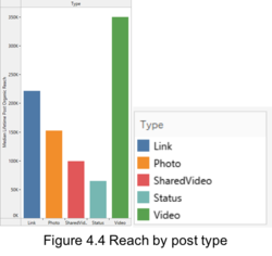
From Figure 4.4 above, we can see that on average, video posts generated notably better performance as compared to the other media type. This observation still holds for most industries even when we drill down the analysis to individual advertiser’s industry level (Appendix 1).
Comparison of the Performance of Paid and Unpaid Post
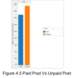
By looking at post reach of paid and unpaid posts, unpaid posts generally perform better as compared to paid posts. Unpaid post performance is 14.93% better than paid post performance. This may be due to the nature of paid post being more relatable and humorous. Hence, SGAG may consider to craft paid posts in such manner to help in generating more reach for paid posts.
Reach of Paid Post by Industry
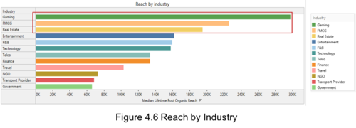
From Figure 4.6, the top 3 best performing advertiser’s industries are Gaming, FMCG and Real Estate. However, upon further investigation, some of the advertiser industries do not actually place a lot of advertisements with SGAG. For instance, the top performing industry which is Gaming, only contain 1 advertiser. As such, these industries may have high performance due to its low number of advertisers and advertisements. To better gauge the performance of the advertiser’s industries, we excluded industries which comprise of only 1 advertiser and as seen in Figure 4.7, the result was significantly different and the top 3 best performing industry will then be FMCG, Entertainment and F&B.
Top Posts with Most Reach
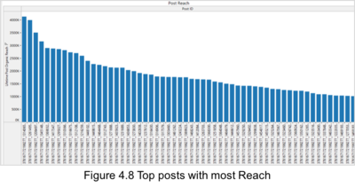
Based on our discussion with SGAG, Reach is an important factor in deciding the performance of a post. Higher Reach indicates that the post is seen by a larger audience base. Hence, examining the top posts with most reach will allow us to know the different types of post that attracts the most audience. Figure 4.8 illustrates the Top Reach generated by SGAG Facebook posts over the past year. The top performing post reaches over 4 Million audiences which is 8 times the total likes of SGAG Facebook page. Meanwhile, Figure 4.9 shows us the different type of posts that generated the highest reach. These posts are relevant to the current happening events or trends, as well as related to the pride of Singapore.
Top Posts with Most Engagements
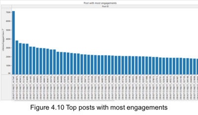
Posts with most engagements are posts that generate discussion amongst the audience, these posts spark the interests of the audience, such that people keep interacting with the posts and share it to their friends. Engagements allow the post to reach out to the friends of people that are interacting with the posts and thus, will potentially generates higher reach. Hence, engagements of a post are also an important indicator of the post’s performance. Figure 4.10 depicts the posts with top engagements, while Figure 4.11 represents the instances of such posts. While the 3 posts shown in Figure 4.11 are of different topics, a noteworthy observation is that all of the 3 posts are considered as humorous posts.
Posts with Most Negative Feedbacks
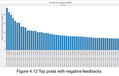
As seen in Figure 4.12, the amount of negative feedbacks received from SGAG’s audience are not very significant, most of the posts received lesser than 100 negative feedbacks and the post with most negative feedbacks received 237 feedbacks. While the figure of negative feedbacks is not as noticeable as compared to the number of engagements and reach that SGAG have, posts with negative feedbacks are able to show SGAG the type of posts that people dislike and will be able to help them in deciding what kind of Facebook post to craft in the future. From Figure 4.13, the post with most negative feedbacks features a picture that is perceived as indecent, while it is actually a dog cartoon character. The reason of why this specific post generated highest negative feedbacks among all the posts this past year may be due to the preview picture deemed inappropriate to be shown in social media platform like Facebook as kids of any age will be able to enter the social media platform easily. It is important to note that the next two posts with most negative feedbacks are also posts with relatively high reach and engagements. This is because popular posts appear frequently on people’s timeline and some may find it annoying and repeating. Hence, decided to hide it away from their timeline. As for the last post on Figure 4.13, while most people find it funny, others may see the video as disrespectful act towards our Prime Minister, Mr Lee Hsien Loong, this results in higher negative feedbacks in this post.
Problem Definition
In measuring the performance of SGAG’s Facebook posts, the reach of the post which is defined as the total number of users who have seen a particular post is commonly used among the social media content creators. Nevertheless, it is challenging for them to determine the various components that may possibly affect this KPI with merely human judgement. Thus, an attempt to utilize the multiple linear regression analysis in examining these factors influencing the KPI will be discussed in the following section.
Analysis Methodology
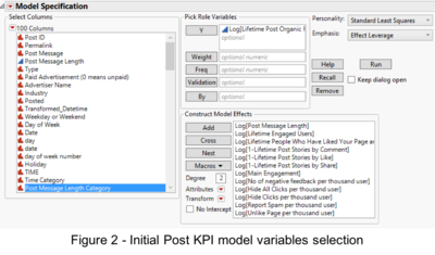
As mentioned previously, Multiple Linear Regressions can be developed using the Fit Model platform of JMP Pro by selecting the response variable (Y axis) which is Post’s reach (Lifetime Organic Post Reach) and the explanatory variables (X axis) which comprises of various continuous variables such as Main Engagement and Negative Feedbacks. Categorical variables will be added to the model once multicollinearity is eliminated from the model.
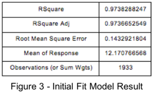
As seen from Figure 3, 97% of variability of the response variable can be explained by the explanatory variables. High R-Square indicates high accuracy of the model. Nonetheless, multicollinearity will need to firstly be examined in order to attain the true factors affecting the KPI.
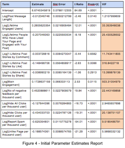
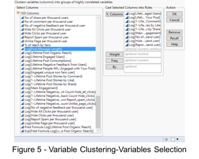
From Figure 4 above, the highlighted columns such as Lifetime Engaged Users and Hide Clicks per thousand user indicate variables with VIF of larger than 8. These variables will be re-selected through the use of variables clustering analysis to eliminate the multicollinearity.
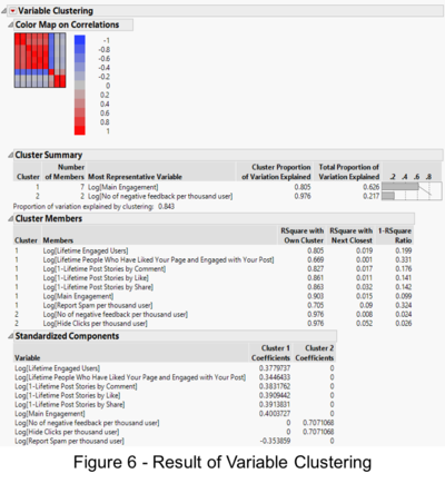
As shown in Figure 6, there were two clusters formed and the representative variables are Main Engagement and No of negative feedback per thousand users. Hence, other variables will be removed from the model and the model will be re-run and further evaluated.
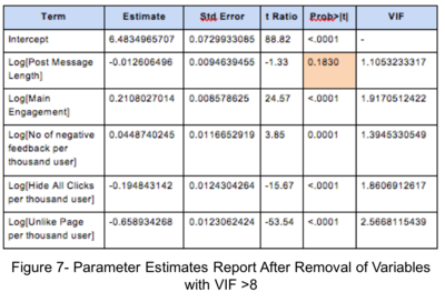
From Figure 7, the remaining independent variables are those with VIF < 8. After eliminating multicollinearity from the model, we will now attempt to filter insignificant factors from this model. As explained previously, variables with p-value (Prob>|t|) of larger than 0.05 are considered as insignificant and the highlighted factor (Post Message Length) have a p-value of 0.18. Therefore, will be removed from the model to improve the true accuracy of the model. Afterwhich, categorical variables such as type and public holiday will also be included to the model.
Results
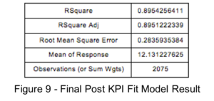
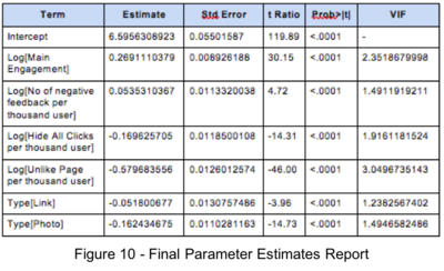
The final model and its reports can be seen from Figure 9 and 10. In this model, 89.5% of the variability of the response variable (Post Reach) can be explained by the various independent variables (Main Engagement, Number of Negative Feedbacks per thousand user, Hide All Clicks per thousand user, Unlike Page per thousand user, Type). The VIF of the explanatory variables are lesser than 8, indicating no multicollinearity exists and p-value of all variables are lesser than 0.0001 indicating strong it is a strong model.
Equation representing the relationship between the dependent variable and the independent variables can be written as such:
Post Reach = 6.60 (intercept) + 0.27 ( Log[Main Engagement] ) + 0.05 ( Log[No of negative feedback per thousand user] ) - 0.17 ( Log[Hide All Clicks per thousand user] ) - 0.58 ( Log[Unlike Page per thousand user] )+ Match( Type )("Link" → -0.05, "Photo" → - 0.16, "Video" → 0.21)
To further examine the effects of the independent variables on the dependent variable, the equation which consists of values which were previously transformed by logarithm function is converted back to the original values through the use of exponential function. Through the profiler seen in Figure 11, we will be able to see the degree of linearity of each independent variable towards the dependent variable, as well as the degree of sensitivity of the response variable to the adjustments of the explanatory variables.
