Difference between revisions of "Three horrible guys Data"
| Line 165: | Line 165: | ||
The table illustrates the category and rationale of the roads classified as either delivery route or non delivery route. | The table illustrates the category and rationale of the roads classified as either delivery route or non delivery route. | ||
| + | |||
| + | {| class="wikitable" | ||
| + | |- | ||
| + | !Type of Road !! Category !! Rationale | ||
| + | |crossing ||non_delive ||For pedestrians | ||
| + | |cycleway ||non_delive ||Assuming delivery riders are motor riders so cycleway is not applicable. Can be changed in future if bicycle is a relevant method for delivery | ||
| + | |} | ||
| + | footway non_delive For pedestrians | ||
| + | living_street non_delive For pedestrians | ||
| + | motorway non_delive High Speed expressway, assuming that Pizza Hut deliver within its own trade area, therefore there is no need for it to access motorway | ||
| + | path non_delive For pedestrians | ||
| + | pedestrian non_delive For pedestrians | ||
| + | steps non_delive For pedestrians | ||
| + | trunk non_delive For pedestrians | ||
| + | trunk_link non_delive For pedestrians | ||
| + | unclassified non_delive For pedestrians | ||
| + | primary delivery_r Road can be used for delivery | ||
| + | pimary_link delivery_r Road can be used for delivery | ||
| + | residential delivery_r Road can be used for delivery | ||
| + | secondary delivery_r Road can be used for delivery | ||
| + | secondary_link delivery_r Road can be used for delivery | ||
| + | service delivery_r Road can be used for delivery | ||
| + | tertiary delivery_r Road can be used for delivery | ||
==<div style="background: #8b1209; padding: 15px; line-height: 0.3em; text-indent: 15px; font-size:18px; font-family:Helvetica"><font color= #FFFFFF>Comments</font></div>== | ==<div style="background: #8b1209; padding: 15px; line-height: 0.3em; text-indent: 15px; font-size:18px; font-family:Helvetica"><font color= #FFFFFF>Comments</font></div>== | ||
Revision as of 02:05, 22 November 2019
Contents
- 1 1. Geometry and Coordinate Reference System
- 2 2. Extracting each POI from the different shp files
- 3 3. Formation of polygons for each branch to align to ppt slides' trade area
- 4 4. Creation of competitors' POI
- 5 5. Aggregation of count of each POI to each trade area (Script)
- 6 6. Extracting Sales Data
- 7 7. Extraction of Population Data
- 8 8. Selection of Roads for Shortest Path Analysis
- 9 Comments
1. Geometry and Coordinate Reference System
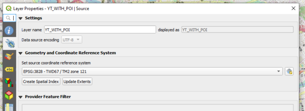
Prior to performing data transformation for the above data, all data layers have to adhere to the same reference system used by Taiwan to use the same unit measurement system. Hence, all data layers utilise the EPSG:3828 Reference System.
Information on 3828 Reference system: https://epsg.io/3828
2. Extracting each POI from the different shp files
We are given the following POIs to extract:
- ATM
- Bank
- Bar or Pub
- Bookstore
- Bowling Centre
- Bus Station
- Business Facility
- Cinema
- Clothing Store
- Coffee Shop
- Commuter Rail Station
- Consumer Electronics Store
- Convenience Store
- Department Store
- Government Office
- Grocery Store
- Higher Education
- Hospital
- Hotel
- Medical Service
- Pharmacy
- Residential Area/ Building
- Restaurant
- School
- Shopping
- Sports Centre
- Sports Complex
- Train Station
- Night Life
- Industrial Zone
- Speciality Store
- Performing Arts
These POIs have to be extracted by finding their respective Facility Type in the shp files provided.
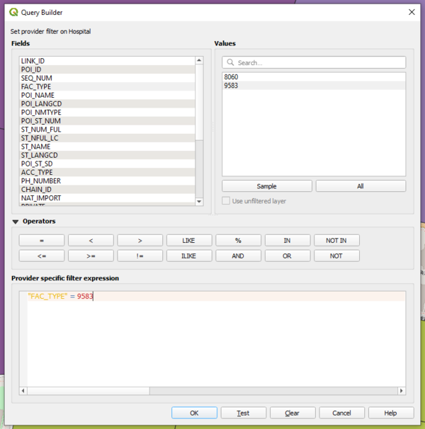
For example, Facility Type of 9583 was filtered using the filter function in QGIS and exported as a layer to the geopackage.
3. Formation of polygons for each branch to align to ppt slides' trade area
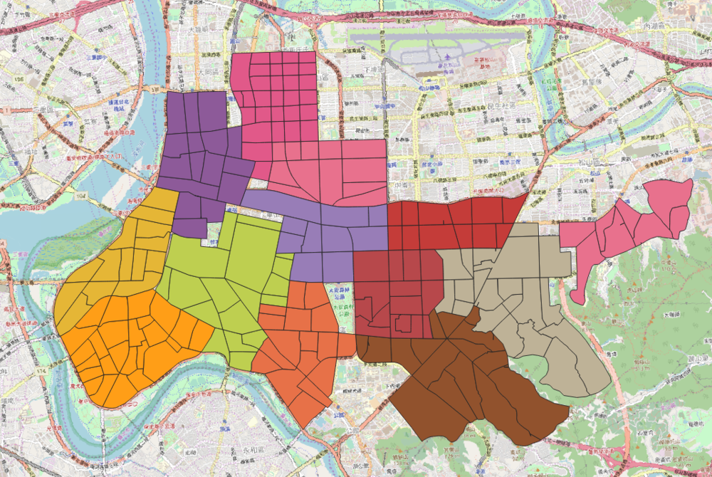
As the trade areas are predefined from the ppt slides, we have to manually digitalise the trade area for each of the outlets. QGIS tools were used in the process: Split Features, Merge Features and our artistic skills. Moreover, we have added the store codes and area code given by the ppt slides so that we can easily identify these polygons.
Below is the generated polygons for all of our trade area.
4. Creation of competitors' POI
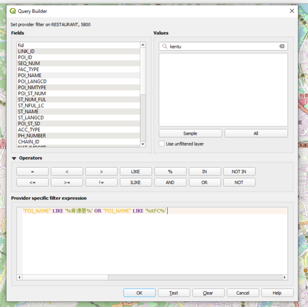
5 Competitors are identified from the powerpoint slides and they are Domino's Pizza, Napolean, Mcdonalds, Kentucky Fried Chicken (KFC) and MosBurger. These data points are crucial in our analysis as they may have a correlation with the sales data. Hence, these competitors store locations must be extracted from the “Restaurant” SHP file. After extraction, they are exported as layers in the geopackage to be used for aggregation.
For example, KFC is filtered from “Restaurant” as shown below:
5. Aggregation of count of each POI to each trade area (Script)
After all the POIs have been extracted from the respective SHP files, the number of points for each POIs must be aggregated using “Count Points in Polygon” tool in QGIS.
However, the batching processing tool is unable to append each newly created column to an existing GeoPackage. Hence, a python script was written and ran under QGIS’s Python Console. It mainly utilised “qgis:countpointsinpolygon” function. Example of the script is shown below:
Learn more about the function here: https://docs.qgis.org/2.8/en/docs/user_manual/processing_algs/qgis/vector_analysis_tools/countpointsinpolygon.html
After the aggregation of POIs into each trade area, below is the screenshot of the columns for a particular trade area.
Since all POIs are contained in their own geopackage, we need to find a way to merge these geopackages into one. Gladly, we have the OSGeo4W Shell. It allows us to run shell commands to merge these geopackages.
First, open the OSGeo4W Shell and cd to the directory that has the master geopackage (Taiwan_stores0x.gpkg) we want to merge into.
cd C:\Users\.......\Project\data\GeoPackage
And as all the layers in each geopackage is named as Taiwan_stores37, I want to rename them to their respective area. The test folder contains all the geopackages that I want to merge.
for %f in (./test/*.gpkg); do ogrinfo ./test/%f -sql "ALTER TABLE Taiwan_stores37 RENAME TO %~nf"
Lastly, the below command append and merges all the geopackages in the test folder into Taiwan_stores0x.gpkg.
for %f in (./test/*.gpkg); do ogr2ogr -f "format" -append ./Taiwan_stores0x.gpkg ./test/%f
6. Extracting Sales Data
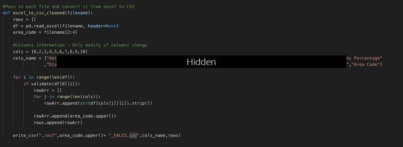
We obtained raw sales data which was generated from the company's Sales system. These were provided to us in a report format which was not directly importable into QGIS. There were over 200 data entries for each store, and it would have been impossible to do it manually. Therefore, we wrote 2 scripts that were used to extract key information from the report and automated the output for the directory.
Although we could not directly import the reports into QGIS, there was a pattern in each report which allow us to easily parse and obtain key information which can be outputted into 2 different types of output: Daily Sales Data, Regional Sales Data for a Year.
Both scripts were written in Python. We found that valid rows have date on its left for the Daily Sales Data. Therefore, we made us of this pattern to export the daily sales data into a separate CSV. In another similar script, we identified that once a certain word is encountered in the first column, any rows after that consisted of Regional Sales data and therefore made us of that fact to write a second script for a different output.
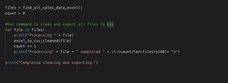
This method is then called in both scripts to enable all the Reports in the directory to be processed and outputted as a separate CSV in another directory. This allowed us to easily distribute the Regional Sales Data to the other groups who were working on different regions.
7. Extraction of Population Data
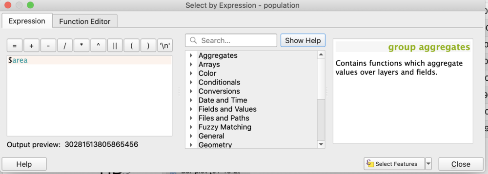
The above is a sample of the population data where we have the Total Population, Total Land Area and Population Density in District X. The population for each store can be created by calculating the proportion of area for each trade area pertaining to the subzone. Firstly, each store area is calculated using the “$area” formula.
The population density is then calculated using the following formula: Area of trade area polygon in District X / Total Land Area in District X * Population Density in District X
From the population count, the population density is then normalised using the following formula:
(x - min) / (max - min)
Below is the final output of the normalised population density in the GeoPackage layer:
8. Selection of Roads for Shortest Path Analysis
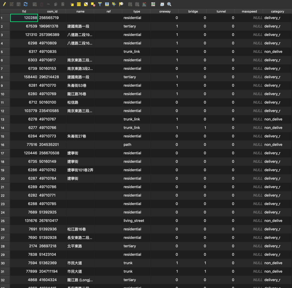
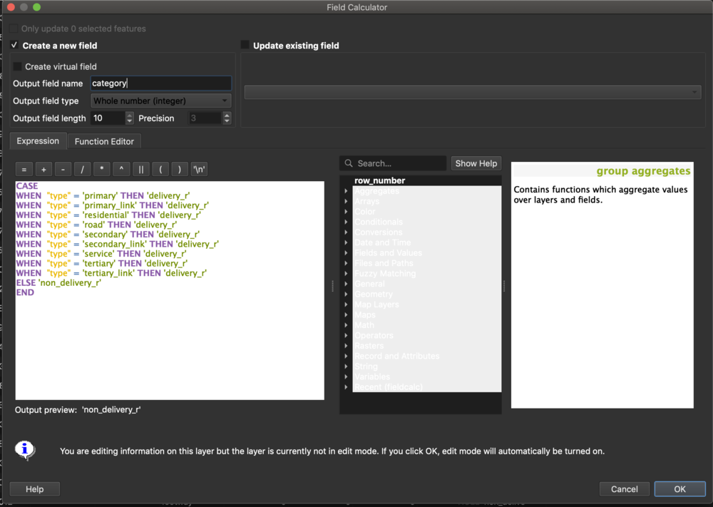
The Road layer that we retrieved online contained many other irrelevant roads that cannot be used as part of the delivery route. Therefore, there was a need for us to filter the roads to be used for further analysis. We added an additional column called category that classify the part of the road based on whether it can be used as a delivery route or non-delivery route.
This is done using the Field Calculator to derive the new values for the category using CASE and WHEN
The table illustrates the category and rationale of the roads classified as either delivery route or non delivery route.
| Type of Road | Category | Rationale | crossing | non_delive | For pedestrians | cycleway | non_delive | Assuming delivery riders are motor riders so cycleway is not applicable. Can be changed in future if bicycle is a relevant method for delivery |
|---|
footway non_delive For pedestrians living_street non_delive For pedestrians motorway non_delive High Speed expressway, assuming that Pizza Hut deliver within its own trade area, therefore there is no need for it to access motorway path non_delive For pedestrians pedestrian non_delive For pedestrians steps non_delive For pedestrians trunk non_delive For pedestrians trunk_link non_delive For pedestrians unclassified non_delive For pedestrians primary delivery_r Road can be used for delivery pimary_link delivery_r Road can be used for delivery residential delivery_r Road can be used for delivery secondary delivery_r Road can be used for delivery secondary_link delivery_r Road can be used for delivery service delivery_r Road can be used for delivery tertiary delivery_r Road can be used for delivery
Comments
Feel free to leave comments / suggestions!

