Difference between revisions of "SMT201 AY2019-20T1 EX1 Renata Dharma"
Renatad.2018 (talk | contribs) |
Renatad.2018 (talk | contribs) (→Part 2) |
||
| Line 66: | Line 66: | ||
! Stage 1 | ! Stage 1 | ||
|- | |- | ||
| − | | | + | | In the first stage, these data files were sourced: |
| + | # 1. Singapore Residents by Planning Area/Subzone, Age Group and Sex, June 2000 - 2018 from Department of Statistics Singapore | ||
| + | # 2. Singapore Master Plan 2014 Subzone and Planning Area 2014 boundary data from data.gov | ||
| + | |||
| + | Inside the dataset: | ||
| + | # The relevant features include Population, Age Group, Planning Area, Subzone, Time (in years) | ||
| + | |||
| + | Data Processing: | ||
| + | # Due to the absence of a common primary key between the two data sets, upper("SZ") was implemented through field calculator to generate the primary key for dataset (1). | ||
| + | # To filter dataset(1) for relevant years, QueryBuilder was used to filter where time=2010 or time=2018. | ||
| + | |||
| + | {| class="wikitable" | ||
| + | |- | ||
| + | ! Time=2010 !! Time=2018 | ||
| + | |- | ||
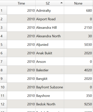
| + | | [[File:2010 total pop.png|300px]] <br> | ||
| + | Table 1.1 generating Subzone, Population Count, Time respectively <br> | ||
| + | Layer: SZ_SumPop2010 | ||
| + | || | ||
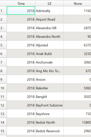
| + | [[File:2018 total pop.png|300px]] <br> | ||
| + | Table 1.2 generating Subzone, Population Count, Time respectively <br> | ||
| + | Layer: SZ_SumPop2018 | ||
| + | |} | ||
| + | |||
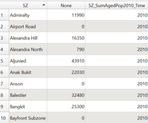
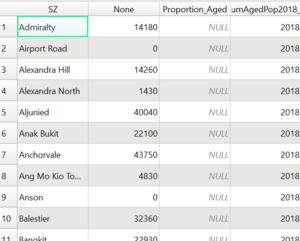
| + | Using field calculator to select AG for 65 and above, and also using a plugin called Group Stats, the AG column was aggregated into 65 and above, so as to determine the frequency of aged population per subzone. | ||
| + | |||
| + | {| class="wikitable" | ||
| + | |- | ||
| + | ! Time=2010 !! Time=2018 | ||
| + | |- | ||
| + | | [[File:2010 total aged pop.png|300px]] <br> | ||
| + | Table 2.1 showing Aged Population Frequency at each Subzone in 2010 <br> | ||
| + | Layer: SZ_SumAgedPop2010 | ||
| + | || [[File:2018 total aged pop.png|300px]] <br> | ||
| + | Table 2.2 showing Aged Population Frequency at each Subzone in 2018 <br> | ||
| + | Layer: SZ_SumAgedPop2018 | ||
| + | | | ||
|- | |- | ||
! Stage 2 | ! Stage 2 | ||
Revision as of 19:43, 15 September 2019
Part 1
| Stage 1 |
|---|
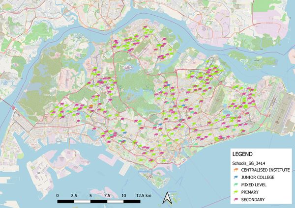
In the first stage, 1 data file was sourced:
Inside the datasets:
Data processing:
Visualising the layers:
|
| Stage 2 |
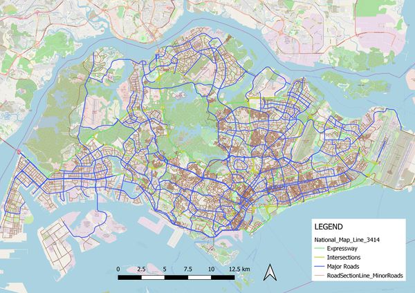
In the second stage, 2 data files were sourced:
Inside the datasets: From the Road Selection Line dataset, the entire country's Road System Network was obtained, which included the major and minor roads. From the National Map Line dataset, major features for national map data represented in polyline form were found. Data includes road data like expressway, major roads, international boundary and contour lines. Data Processing: The data were categorized into 3 different colours: yellow, green and blue. As the island contour lines did not apply to this stage of the Take-Home Exercise, it has been removed so that only Major Road, Expressways and Intersections were shown. Visualising the layers: The vector representing Major Roads, Expressways and Intersections have been modified to a larger width so that it is more obvious on the map. By making use of layer ordering, by placing (2) over (1), the non-overlapping vectors would represent the Minor Roads. |
| Stage 3 |
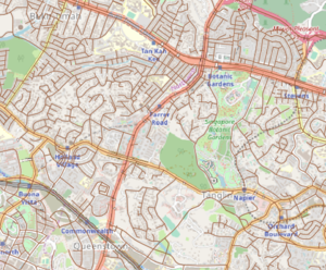
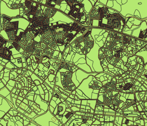
In the 3rd stage, 1 file was sourced:
Data Processing: The layer was modified to ensure consistent projection. Visualising the layers: The layers' dependent visibility was scaled to a minimum of 1:50000. This ensures that the map does not take too long to render while it was initially opened and that only meaningful base maps were used. At a lower scale, there is a need to see the individual roads and buildings surrounding lanes or roads. However, at a higher level, it is better for the specific area in Singapore to be seen so as to aid analyzing frequency base on each neighbourhood. The image shows a map view at 1:50000 and another at map view 1:49999, where the planning area base map is visible. <break> |
