IS428 AY2019-20T1 Assign Tommy Johnson DataAnalysisTransformation
Before moving on to the analysis, it is essential to clean and transform the raw data so that I can bring value to the analysis. In the zipped file, I am given 3 raw data sets namely:
- MobileSensorReadings.csv - contains the sensor readings of different mobile sensor Ids over a period of time and its locations
- StaticSensorReadings.csv - contains the sensor readings of different static sensor Ids over a period of time
- StaticSensorLocations.csv - contains the different static sensor Ids with its locations
I will be using Tableau Prep to clean and transform the data. It is a new feature provided by the Tableau. The following section will explain step by step on how I prepare the data sets.
Contents
1. Combine the Static sensor readings and locations
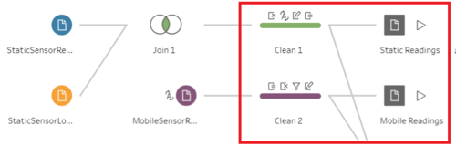
The first step is to combine the two csv files of static into one. This is to create a tidier data (Tall and skinny structure). I use Join to combine the columns from two different files into one.
2. Create a calculated field for Static and Mobile sensor Ids
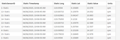
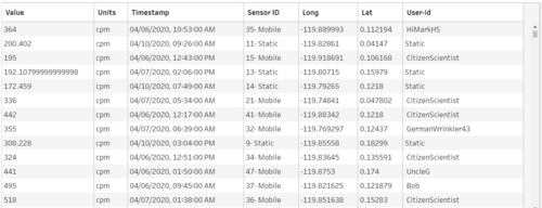
The next step is to concatenate "- Static" or "- Mobile" at the back of the sensor Ids with the [Sensor-id] + "- Mobile" or [Sensor-id] + "- Static" calculated fields. This is because I realize that the static sensor Ids have the same Id number although they are referring to different records. Hence, this is done to avoid confusion at the later part. The final output will be as follow.
Static Sensor
Mobile Sensor
3. Combine the static and mobile sensor data into one
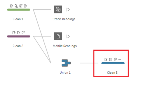
The next step is to combine the static and mobile sensor data into 1 file. This will be the working file that I am going to use in Tableau. I use Union because I am just going to append more rows. After that, I will still need to clean the data to remove any duplicate columns so that all columns are arranged.
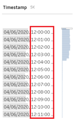
4. Aggregated the Timestamp by 1 minute interval
Using the following formula, I aggregate the timestamp by 1 minute interval
DATETIME(INT([Timestamp]) + (INT(FLOAT([Timestamp]) % 1 * (60*24)) / (60*24)))
DATETIME(INT([Timestamp]) : Retain the datetime of the timestamp
(INT(FLOAT([Timestamp]) % 1 * (60*24)) / (60*24))) : A calculation to create a 1-minute interval. ([60 minute] / [desired minute interval] * [24 hour])
After that, i deleted the original Timestamp from the raw data.
5. Aggregated the Value based on the Timestamp
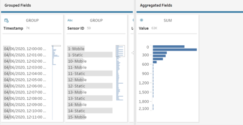
After aggregated the timestamp, I sum all the measuring readings for that particular sensor ID within that 1 minute interval. For example, 12 counts of readings level for Sensor ID 1 across different seconds. I summed the 12 counts and created 1 row within that minute. This will reduce the number of rows in the data set. Hence, create a faster running time.
The final Workflow will look like this:


