IS428 AY2019-20T1 Assign Ng Kai Ling Bernice Questions
Contents
- 1 Questions & Observations
- 1.1 Q1) Visualize radiation measurement and characterize changes over time.
- 1.2 Q2) Use visual analytics to represent and analyze uncertainty in the measurement of radiation across the city.
- 1.2.1 A) Compare uncertainty of the static sensors to the mobile sensors. What anomalies can you see? Are there sensors that are too uncertain to trust?
- 1.2.2 B) Which regions of the city have greater uncertainty of radiation measurement? Use visual analytics to explain your rationale.
- 1.2.3 C) What effects do you see in the sensor readings after the earthquake and other major events? What effect do these events have on uncertainty?
- 1.3 Q3) Given the uncertainty you observed in question 2, are the radiation measurements reliable enough to locate areas of concern?
- 1.3.1 A) Highlight potential locations of contamination, including the locations of contaminated cars. Should St. Himark officials be worried about contaminated cars moving around the city?
- 1.3.2 B) Estimate how many cars may have been contaminated when coolant leaked from the Always Safe plant. Use visual analysis of radiation measurements to determine if any have left the area.
- 1.3.3 C) Indicated where you would deploy more sensors to improve radiation monitoring in the city. Would you recommend more static sensors or more mobile sensors or both? Use your visualization of radiation measurement uncertainty to justify your recommendation.
- 1.4 Q4) Summarize radiation measurement and compare static sensor network to mobile sensor network.
- 1.5 Q5) The data for this challenge can be analyzed either as a static collection or as a dynamic stream of data, as it would occur in a real emergency. Describe how you analyzed the data - as a static collection or a stream. How do you think this choice affected your analysis?
- 2 Appendix
- 2.1 Figure 1.1.1 Radiation measurement fluctuation
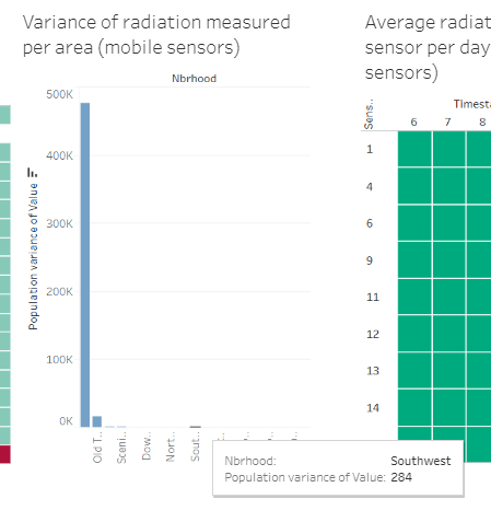
- 2.2 Figure 1.1.2 Population variance of radiation fluctuation per location (mobile sensors)
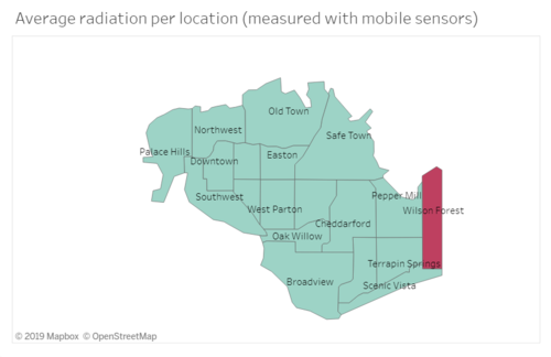
- 2.3 Figure 1.1.3 Average radiation across a period of time
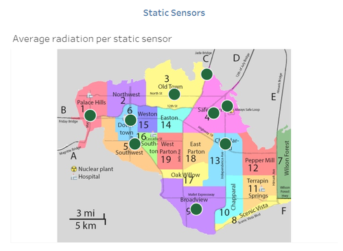
- 2.4 Figure 2.1.1 Location of all static sensors
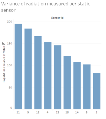
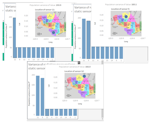
- 2.5 Figure 2.1.2 Population variance of radiation fluctuation per location (static sensors)
- 2.6 Figure 2.2.1 Average radiation across a period of time
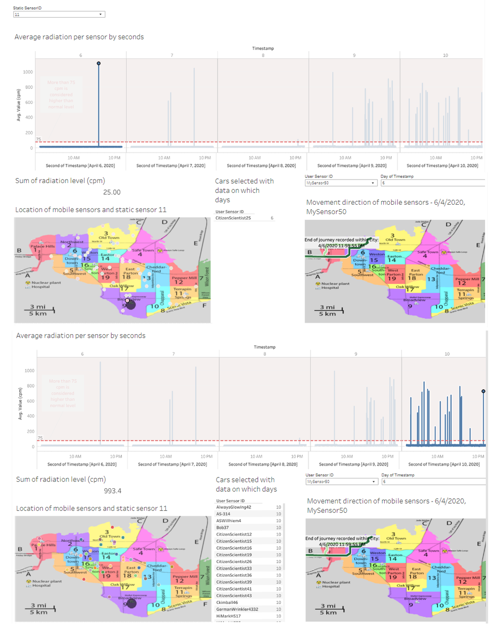
- 2.7 Figure 3.1.1 Radiation contaminated cars
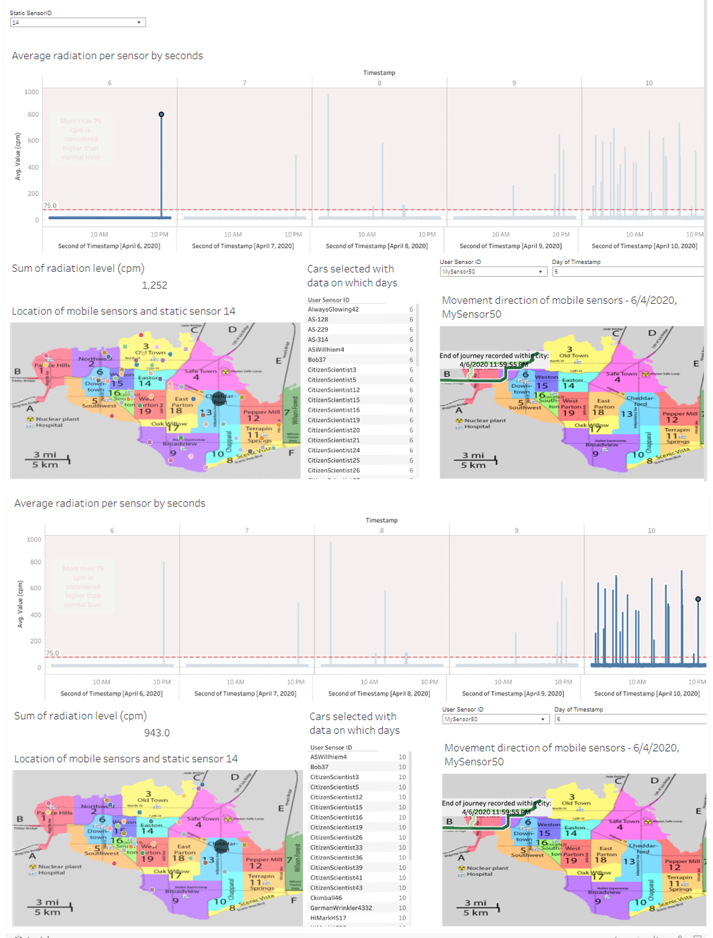
- 2.8 Figure 3.1.2 No cars nearby static sensors when measured high radiation
- 2.9 Figure 3.2.1 Contaminated car exits area
Questions & Observations
Q1) Visualize radiation measurement and characterize changes over time.
- Generally, the frequency of radiation increases as in the later part of the available period (refer to Figure 1.1.1).
- Radiation measurements fluctuate heavily (refer to Figure 1.1.2) which can be caused by the air movement in certain directions (towards or away from sensors).
- The locations with sensor readings of high frequency of radiation level above 75 are potential places of contamination.
- Although the average radiation for most places over the entire available period is lower than 75 cpm (refer to Figure 1.1.3), it does not mean that the location is not contaminated. This is because, by looking at Figure 1.1.1, you can still see that the sensors did detect high levels of radiation every now and then.
Q2) Use visual analytics to represent and analyze uncertainty in the measurement of radiation across the city.
A) Compare uncertainty of the static sensors to the mobile sensors. What anomalies can you see? Are there sensors that are too uncertain to trust?
Uncertainty of static sensors:
- Only records the radiation level within receivable area where the sensors are places and hence not representative of the level of radiation in the area. This is especially so where sensors are placed nearer to the borders of the area (refer to Figure 2.1.1).
- Only 9 static sensors are installed. This means that certain areas’ radiation is not measured (refer to Figure 2.1.1).
Uncertainty of mobile sensors:
- Unable to measure the radiation level changes in a single location as the sensors are moving to different areas. Unless it is placed at a location without moving.
- Because it is a moving target, it can bring radiation to the various locations, contaminating the area without being able to measure it.
Anomalies:
- The static sensors have sudden increase and decrease in radiation measurement in a matter of a minute. These measurements should not fluctuate with such big difference (refer to Figure 2.1.2). This makes it difficult to understand the real areas of concerns.
B) Which regions of the city have greater uncertainty of radiation measurement? Use visual analytics to explain your rationale.
The top 3 cities that have greater uncertainty of radiation measurements are Broadview, Old Town followed by Jade Bridge. This is because that they have the biggest population variance value as compared to the rest of the cities (refer to Figure 2.2.1) which means that there is a bigger difference in the fluctuated radiation values measured.
C) What effects do you see in the sensor readings after the earthquake and other major events? What effect do these events have on uncertainty?
Earthquakes could have contributed to the movement of the air, causing the fluctuations of radiation measurement (refer to Figure 1.1.1). With these, it can cause uncertainties on areas of concerns and what actions to take.
Q3) Given the uncertainty you observed in question 2, are the radiation measurements reliable enough to locate areas of concern?
A) Highlight potential locations of contamination, including the locations of contaminated cars. Should St. Himark officials be worried about contaminated cars moving around the city?
Contaminated by cars:
- Downtown
- Old Town
- Broadview
Contaminated locations:
- Jade Bridge
- Palace Hills
- Southwest
- Safe Town
- Cheddarford
- Wilson Forest
St. Himark officials should be worried about contaminated cars moving around the city. This is because, there is a possibility that cars can carry radiation with them wherever it goes. Using the sensors to measure radiation in cpm, you will not know the strength of the radiation as well. From Figure 3.1.1, we can see that when the static sensor in Downtown first measured radiation above 75 cpm, ProfessorSievert’s car was nearby. Thereafter, there wasn’t much cars nearby and the values started to fluctuate even more frequently till the end of available period. This shows that there is a potential that contaminated cars can potentially contaminate the area it went as well.
As for the contaminated locations identified, it was done by checking frequencies of fluctuations and if there were any cars nearby (refer to Figure 3.1.2).
B) Estimate how many cars may have been contaminated when coolant leaked from the Always Safe plant. Use visual analysis of radiation measurements to determine if any have left the area.
Estimated 4 cars to be contaminated. Specifically, Ckimball (car with sensor ID 46), CitizenScientist (car with sensor ID 19, 20, 25) and MySensor (car with sensor ID 7) cars. From Figure 3.1.1, you can see that the very first radiation measurement took a sudden increase, CitizenScientist’s car with sensor ID 19 and 20 were nearby Downtown city. The same goes to CitizenScientist’s car with sensor ID 25 being nearby to Broadview, and MySensor’s car with sensor ID 7 near Old Town city. There are instances where contaminated cars left by Wilson Forest Highway (CitizenScientist’s car with sensor ID 25), Jade Bridge (Ckimball’s and MySensor’s car with sensor IDs 46 and 7 respectively). Taking Figure 3.2.1 as an example, there is measurements of radiation moving towards each of the mentioned above and coming back after a few hours. Hence a possibility that the contaminated car could have left the area and brought the contamination to other areas.
C) Indicated where you would deploy more sensors to improve radiation monitoring in the city. Would you recommend more static sensors or more mobile sensors or both? Use your visualization of radiation measurement uncertainty to justify your recommendation.
Since mobile sensors can move from one place to another, it will be difficult to measure changes over time. You can also refer to Figure 1.1.1 to see how the radiation level can fluctuate over time which might be due to wind directions and so having static sensors are not enough. Hence, I would suggest the use of both static and mobile sensors. I would place 1 – 3 static sensors to areas depending on the size of the area. For example, I would put 3 static sensors spread out in areas like Broadview and Safe Town. Also, place the sensors not near the borders but spread out. By doing so can improve coverage of the area. This can also help to monitor the radiation levels over time. I would also use 1 – 2 mobile sensors to even improve on the coverage in each area. However, I would only dispatch mobile sensors to move within the area only as there could be a risk of contaminated cars contaminating the area with radiation as well (refer to Figure 3.1.1). For example, mobile sensor 1 can only move within Palace Hills.
Q4) Summarize radiation measurement and compare static sensor network to mobile sensor network.
Summarize the state of radiation measurements at the end of the available period. Use your novel visualizations and analysis approaches to suggest a course of action for the city. Use visual analytics to compare the static sensor network to the mobile sensor network. What are the strengths and weaknesses of each approach? How do they support each other? (Limit your response to 6 images and 800 words)
Evacuate those who need medical help to hospitals in Terrapin Springs and Southon as these 2 areas are not suspected to be heavily contaminated by radiation. Meanwhile, modify the sensor network allocation to improve the monitoring.
As mentioned in question 3, the course of action would be dispatching 1 – 2 mobile sensors within each area and deploy 1- 3 static sensors in each area depending on the size of the areas.
If we have a static sensor network all over the country, it will be difficult to get an accurate gauge of the area’s condition as static sensors cannot get the measurement of certain parts of the area (refer to Figure 1.1.1 for the fluctuated measurement of radiation). However, if we have mobile sensor network all over the country, it will be difficult to understand the radiation changes over time of a part of the area. Furthermore, as mentioned previously, cars can potentially get contaminated and cause the area it went to, to be contaminated as well (refer to Figure 3.1.1).
However, having a combination of both can help provide data to support each other. With the static data, it can give an overview of the radiation changes over time. On the other hand, mobile data can help to see if other parts of the area radiation level. Having these 2 in place, you can use mobile data to identify cars that are contaminated while justifying whether the static data is reliable or not. With this hybrid sensor network in place, it can help to identify the areas of concern and actionable to the situation.
Q5) The data for this challenge can be analyzed either as a static collection or as a dynamic stream of data, as it would occur in a real emergency. Describe how you analyzed the data - as a static collection or a stream. How do you think this choice affected your analysis?
I used the data as a dynamic stream. This is because, the main idea is to identify the radiation changes within the area to help the management team to make better decisions to evacuate, cleanup or further monitor the situation. While using dynamic stream of data, I analyzed the direction which cars (refer to Figure 3.2.1), be it contaminated or not, is moving to which direction and if it left the area or not. Furthermore, I have shown latest areas of concern (refer to Figure 1.1.3) as the dynamic data are being fed into the dashboard. This will give the management team a timely information about what action to take.
Appendix


