Business Mafia Proposal

Contents
- 1 Project Motivation
- 2 Project Objective
- 3 Data Sources
- 4 Literature Review
- 5 Our Methodology
- 6 Project Storyboard
- 7 Application Overview
- 8 Our Findings
- 9 Reflecting on our project
- 10 Project Timeline
Project Motivation
A significant proportion of Airbnb hosts rent out portions of their own homes to generate additional side income. Instead of relying on a robust approach when setting prices, they tend to do so intuitively, relying on gut feeling. Our group hopes to offer these homeowners an alternative way to price their listings - by setting prices based on their listing's geographical location.
However, the primary challenge here is simplifying and summarising the technical, complex analytics techniques into layman terms; it would require breaking down the technical jargon associated with it. In order to carry this out effectively, we built an RShiny Application which will guide hosts (both current and potential) systematically through the thought process. This would allow owners to not only derive at a proposed listing price, but also better understand our thought process and methodology behind the derivation of the price.
Project Objective
Through our project, we aim to:
- Deepen our understanding on the spatial relationships between various key locations and Airbnb listings in Downtown Seattle to determine how a listing's location affects the listing prices
- Build RShiny application that will allow everyone to have access to our work and being able to customise the parameters to suit their own needs better
- Through the use of Local Geographical Weighted Regression (GWR) Model, we hope to help Airbnb owner(s) determine the better pricing for their listing(s)
- Through the use of Spatial Point Pattern Analysis, allow hosts to visualise and understand their listing's surroundings better - the different types of listings surrounding them and the type of amenities they offer.
Data Sources
| Data | Source | Data Description | Source URL | Data Type |
|---|---|---|---|---|
Literature Review
Literature Sources:
- https://towardsdatascience.com/airbnb-rental-listings-dataset-mining-f972ed08ddec
- https://wiki.smu.edu.sg/18191isss608g1/Group01_Proposal
- https://www.researchgate.net/profile/Ben_Miller6/publication/225322212_A_comparison_of_methods_for_the_statistical_analysis_of_spatial_point_patterns_in_plant_ecology/links/02e7e533e0ff93e167000000/A-comparison-of-methods-for-the-statistical-analysis-of-spatial-point-patterns-in-plant-ecology.pdf
Literature Review 1: Airbnb Rental Listings Dataset Mining
Literature's Objective: An exploratory analysis of Airbnb's Data to understand the rental landscape in New York City
- NYC's data was also obtained from Inside Airbnb and it contains the same three tables as ours, except that it was for New York City
- Listings.csv - contains 96 detailed attributes for each listing. Some of the attributes are continuous (i.e. Price, Longitude, Latitude, ratings) and others are categorical (Neighbourhoods, Listing_type, is_superhost) which is used for the analysis
- Reviews.csv - Detailed reviews given by guests with six attributes. The key attributes include date (datetime), listing_id (discrete), reviewer_id (discrete), comments (textual)
- Calendar.csv - Provides details about booking for the next year for each listing. There are four attributes in total, they are: listing_id (discrete), date (datetime), available (categorical) and price (continuous).

This is a screenshot of a paragraph taken off the literature. The context behind this paragraph was that the authors were trying to find out the number of days in a year each listing is made available for booking. Our group ran into a similar problem when analysing our Seattle Airbnb dataset.
Unfortunately, the number of days available for booking by each listing is not made publicly available by Airbnb. We found the method proposed by the authors useful as this was a simple solution that made a good enough estimation for us to gauge the number of days available for booking, and conclude if the listing was highly sought after or if it was one of those listings where it opened it's doors only few times each year.

Furthering on the earlier introduced idea that demand can be gauged from the number of reviews left by guests on their home owners, the authors investigated on how demand changes across three years - 2016 (left most graph), 2017 and 2018 (right most graph). All three graphs showed identical trends that demand across the year picks up. The period of peak demand across all three periods happens during the month of October. After which, demand tends to fall. This is mainly attributed to seasonality factors, as the seasons gradually shifts from Fall to Winter. From this, we can conclude that demand and seasonality in New York City are likely to be related to one another. This is a similar idea that can be looked into when exploring Seattle's Airbnb Dataset.

This graph shows the average listing prices per night for each month across all NYC Airbnbs. The average prices tend to increases as one progresses along in the year and Spikes in December. This pattern is similar to that of demand graph above, except in the months of November and December, where the demand starts falling since end October. Hence, one hypothesis that our group came up with when analysing listing prices and demand rates across months of the year(s) is that Airbnb owners do not take into account demand when setting prices. We attribute this to the lack of holistic pricing model(s) or analysis tool(s) that Airbnb owners do not use to understand demand patterns before determining prices. As most Airbnb owners set out to rent their apartments/rooms out to earn additional income, we believe that most owners set prices based on their intuition. This might likely be the case for Airbnb owners in Seattle as well.

This is the basic interactive graph with all the listing in New York City appearing in a clustered fashion. The user can click on the clusters to see the listing it comprises of. This gives a zoom-in view, more minute view of the landscape. A user can further click on each listing to see details of the listing such as the Listing Name, Host Name, Price of Listing, Property Type and Room Type. This visualisation helps to explore the listing geographically. It gives the overall sense of how the listings are distributed across neighborhood. We can see from the map that maximum listing are clustered around Manhattan and Brooklyn region, followed by Queens, Bronx and the least number of listing are in Staten Island. Click on the thumbnail and it will bring you to the animation!
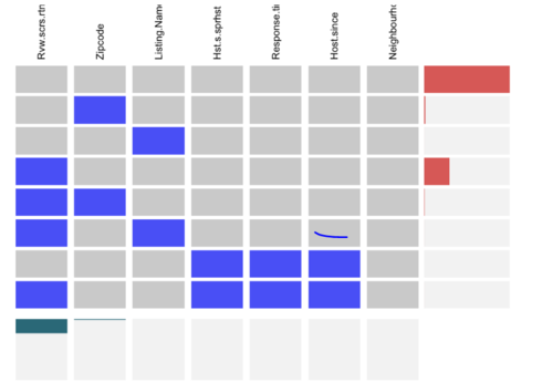
When it comes to dealing with missing values in the dataset, the authors chose to construct a Visna plot to analyse the missing values for the variables they would be using for in their exploratory analysis. To preserve all the information, they imputed or dropped all the rows and columns containing null values when conducting their exploratory data analysis. The variables that they used in their visna plot were:
- host_is_superhost
- neighbourhood_group_cleansed
- host_response_time
- review_scores_rating
- name
- host_since
- zipcode
Few observations were made from this exercise:
- Most rows have no missing values
- reviews_score_rating variable have close to 30% missing fields across all rows
- zipcode, name, host_response_time, host_since and host_is_superhost have only few missing values across all rows and hence are not reflected in the visna plot.
From the plot above, it can be concluded that the Airbnb dataset only contains few missing values which further argues that the analysis done on the data can be performed without much loss of information.
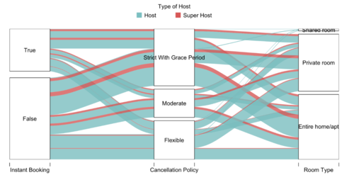
The aim of this analysis is to see if there is any relationship between the different categorical variables in the dataset. The variables under examination are instant_booking, cancellation_policy and room_type. The goal of this study is to see if regular hosts and super hosts have different policies and to examine if there is a correlation among the variables.
Key takeaways from the above chart
- Majority of the listings are not available for instant bookings. Majority of the ones available tend to have strict cancellation policy.
- Properties that are entire homes or apartments tend to have a stricter cancellation policy compared to shared and private rooms. This makes sense as the hosts would want to prevent incurring a huge loss by last-minute cancellations on entire homes/apartments type bookings.
- As the number of shared rooms listings are very few, the line in the graph is very thin. From the graph, all the lines suggest that the shared rooms are available for instant booking and have slightly more flexible cancellation policy.
- Owners of shared rooms are generally regular hosts.
- Based on the features here under inspection, there are no major discrepancies in behaviour between regular hosts and super hosts as they seem to display similar behavior types.
Literature Review 2: Hawk-R-Stall Rental Singapore
Literature's Objective: Determining the market rate for stall rentals and appropriate bidding price for hawker stalls in Singapore
Most of the learnings we gathered from this literature review relates to how we can improve the UI/UX of our project deliverables. It is not only important to do analytics well but it is as important, if not more important to be able to provide the right environment and setup to translate these analytical learnings to just about everyone. Along this line of thinking, our group finds it utmost important to package this learning in a way that is extremely customer-oriented. Thus, a significant portion of mental capacity and resources have been dedicated to creating seamless design UX. This particular project was chosen as the analysis technique used is similar to ours (Geographically Weighted Regression) and that it is a piece of work by someone more experienced then us. Also, by studying work beyond the scope of undergraduate, we are confident that we can pick up fresh, new ideas.
Something different that all other IS415 projects do not have is the 'Project Groups' tab in the project proposal page. This allows for easier navigation between projects as clicking on it allows the user to return to the Project Groups page. Users can more easily exit a group's project and continue on to other projects. We decided to incorporate this feature into our project as well.

The creators of Hawk-R-Stall Rental Singapore have included a User Guide for their RShiny application under the 'Application' tab of their project page. This serves to improve the User Experience (UX) as users can refer to this user guide as and when they have queries regarding the application. This is another feature that we will be incorporating to our project to improve the UX. Ultimately, we want to build applications that are user-friendly and easy-to-use! And a big part of it involves making the UX as seamless as possible!

The authors of Hawk-R-Stall Rental Singapore have included a section under their Project Proposal which addresses the flaws of existing visualisations available. This idea is again something that is not commonly found within undergraduate's work. A considerable amount of resources have been spent on researching into existing solutions. This helps the authors to better their product as they can address pain areas that they find in other tools that are not yet addressed. This is also an idea that we are looking to incorporate, if we can find existing RShiny applications/visualisations that are similar to our group's project.
Literature Review 3: Studies the usage of spatial point pattern analysis methods for the purposes of plant ecology
Plant Ecology, accepted: 10 February 2006 and published online: 30 March 2006
We have chosen this research paper for its broader usage of SPPA in the studies of plant ecology, as well as different statistical method.
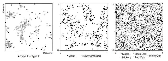
One of the interesting takeaways we caught from this review was its use of a bivariate spatial point pattern analysis on top of a univariate analysis. This usage of two variables helps answer the question if the events of interest are occurring with any respect to separate types of events. The examples used in the review are such as comparing the points of newly emerged plants, and adult plants. Applying to our project’s scope and objective, introducing this analysis brings us one step further in deriving the reasons behind the high Airbnb listing activities in Downtown Seattle; a possible causation.
In the research paper analysis, they had 3 bivariate sets of events used: the Gibbsian point pattern, the Bramble canes event set (newly emerged vs. adults) and the Lansing Woods event set (hickory vs. maple, with other species having smaller grey symbols)
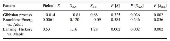
Interpreting the table gave information such as whether the Gibbsian process has a high association value with Dixon's SAA and SBB, and whether Pielou's S is any disimilar from being completely random.
For a second order effect, they used Ripley's K and Neighbourhood Density Function. The overall analysis of the second order concluded that it supports the contingency table analyses.
The usage of a bivariate analysis certainly gives more room for our model to be built upon. Unfortunately, the lack of data hinders us from exploring other events that could suggest the high number of listings in Downtown Seattle. Hence, future research can consider adopting this similar approach to identify a possible reason for dense airbnb listings in Downtown Seattle. Knowing so could inspire new business strategies for home owners or Airbnb itself.
A second interesting finding is the usage of a global and local approach that is combined - the Spatial Analysis by Distance Indices (SADIE)
 |
 |
This approach uses an algorithm in which observed events are iteratively displaced until they achieve a regular arrangement. As seen from the image, these distances are interpreted by totalling up the number of moves each event records until a regular pattern of events are achieved.
Comparing the 2 of the plots, we can see from the top right plot, B, that its lines are not overlapping each other as frequently as the bottom left plot, C. More so, B has a shorter length of lines while C has a larger variance. In addition, observing the directions of the lines in C, they show some radiation outwards and away from distinct clusters.
Similarly, a summary statistic was produced in the literature. Pp is the probability as an extreme aggregation of CSR - offering a statistical result at the same time. Thus, the plots, along with the table, offer another way to observe the clustered distribution of events.
While this technique will not be used, it gives an additional option of interpreting spatial point patterns.
Our Methodology
R Packages used:
- corrplot
- dplyr
- DT
- ggplot2
- ggpubr
- GWmodel
- leaflet
- olsrr
- plotly
- raster
- RColorBrewer
- rgdal
- rsconnect
- sf
- shiny
- shinydashboard
- shinythemes
- sp
- SpatialAcc
- spdep
- tidyverse
- tmap
- tmaptools
General Methodology
- Data wrangling/Data Cleaning
- Extracting only listings in Downtown Seattle
- Extracting out top 12 key attractions in Downtown Seattle
- Computing the street distance from each listing to the 12 different key attractions (Using Open Street Map Server)
- Geographical Accessibility technique as a form of data exploration
- Hansen's Potential Model
- Power function
- Spatial Point Pattern Analysis technique
- First Order
- Second Order
- Geographically Weighted Regression technique for modelling
- Feature Engineering
- Running correlation test obtain correlation of coefficient (R value) - choosing only variables that are significant at 95% confidence level
- Kernel Density Function Used
- Bandwidth used
Geographical Accessibility
Geographical Accessibility refers to the ease of reaching destinations. People who are in highly accessible places can reach many other places quickly while people in inaccessible places can reach fewer places in the same amount of time. In our project, we decided to use Geographical Accessibility technique as an exploratory technique to understand the accessibility of each individual listings. Specifically, we will like to identify areas within Downtown Seattle that have higher accessibility scores and hypothesize that listings within these areas should fetch higher prices.
Hansen's Potential Model

To model geographical accessibility, the Hansen Potential Model was used. To use this model in R, we worked with the ‘SpatialAcc’ library with the ac() function called. There are five parameters that had to be addressed in the ac() function and further paragraphs in this literature will be used to address these five parameters.
Parameter 1: ‘p’
The parameter p is a vector that quantifies the demand for services in each location (origin i). In the case of our project, this refers to all listings within Downtown Seattle. To obtain the population, we filtered for all listings within Downtown Seattle from listings.csv data source. There were a total of 1148 Downtown Seattle listings in our dataset. To quantify the demand from each listing, we looked at the ‘accommodates’ variable. We assumed that the true demand from each listing was represented by the number of guest a listing can accommodate.
Parameter 2: ‘n’
The parameter n is a vector that quantifies the supply of services in each location. We obtained all key attractions within Downtown Seattle from internet sources like tripadvisor.com or planetware.com. A total of 12 key attractions within Downtown Seattle were chosen.

The 12 key attractions are:
- Washington State Ferries
- Olympic Sculpture Park
- Pike Place Market
- Seattle Art Museum
- Benaroya Concert Hall
- Seattle Aquarium
- Seattle Public Library
- Space Needle
- Washington State Convention Centre
- Klondike Goldrush
- Seattle Great Wheel
- Columbia Center
Their corresponding location (latitude, longitude) was extracted from Common Place Name (CPN) dataset taken off City of Seattle Open Data Portal. For the capacity of each key attraction, we searched up the internet to find out either the size of each key attraction or the highest demand the place has ever accommodated. Also, we considered other factors, such as whether the location was enclosed or open spaced, if entry into the attraction requires the visitor to pay entrance fee and whether the attraction was suited only for a specific group of visitors to enter. Taking everything into account, we imputed a new column, ‘capacity’, into our dataset. It represented the supply of service at each location.
Parameter 3: ‘D’
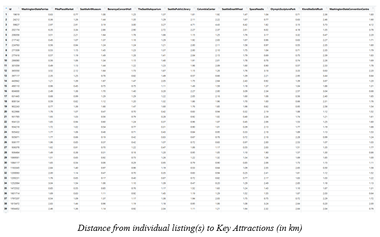
The parameter D is a matrix of quantity separating the demand from the supply. It was a distance matrix using the road network distance. Road Network distance between each listing to all 12 key attractions was calculated using the ‘OSRM’ package. We used Road Network distance and not Euclidean distance (flying distance) as Downtown Seattle was cluttered with city blocks. It was impossible for anyone to travel in a straight line, from any listing to any attraction. Each individual listing’s distance to all 12 key attractions was computed and recorded in a distance matrix. The distance matrix was uploaded into R as a data frame, with 1148 rows by 12 columns.
Parameter 4: ‘power’’

The Distance Decay function is used to reflect the rate of increase of friction in distance. It is used to model how demand decreases as distance increases. In the ac() function, it allows only for the Power function decay and not the exponential function decay. We initially wanted to work with the exponential function instead of the Power function as we believe that visitors will visit still visit these key attractions even if they were a distance away. Hence, the dip in demand as distance increases should not be as steep. Given that only Power function is available, we used a power factor of 0.5 for our model.
Parameter 5: ‘family’’
Family refers to the type of function we used to model Geographical Accessibility. In our case, we used the ‘Hansen’ family.
Spatial Point Pattern Analysis
The use of spatial point pattern analysis (SPPA) is popular in the literatures of plant ecology and the studying of settlement distributions. For a moment in time, SPPA was neglected in geographical analysis purposes. But lately, with the developments of Geographical Information Systems (GIS) and the surge in geo-referenced databases, it has begun to attract renewed interest. Applying to our review, the popularity of Downtown Seattle being densely littered with Airbnb listings makes it worthwhile to study the distribution pattern. From a research perspective, we hope to understand whether the distribution of Airbnb listings follows a random spatial distribution, or a regular or clustered pattern. From an application perspective, the utility of SPPA can help potential Airbnb owners identify where best to locate their next listing location. Some Airbnb hosts may choose to own listings that are away from clusters of Airbnb listings, while some may prefer the company of a crowded Airbnb neighbourhood. Being in either sides triggers different business approaches to optimize the value earned in a listing. This could be in terms of prices, or non-price features such as amenities.
SPPA uses hypothesis testing to statistically determine the behavior of point patterns over a map in one of the following 4 patterns depicted in the image above. It is worth highlighting that a uniform distribution of points has a variance of zero. Whilst random and clustered distributions have variances that are close to one and greater than one respectively.

The null hypothesis usually describes the point patterns as following a complete spatial randomness (CSR). The alternate hypothesis then attempts to describe the points as not following a CSR. The actual set of point patterns are measured against a simulation of point patterns which follow a CSR pattern. A p-value is derived which is compared to the alpha value . If the p-value is lesser than the alpha value, then we reject the null hypothesis of CSR and conclude that the points are not random.
Fundamentally, the SPPA is made of 2 forms of analysis - the first and the second order effect. Each has its own scopes which delivers separate types of observations. It is crucial to note that isolating the results of each is not a recommended approach as both are jointly used to arrive at a reasonable conclusion.
First Order
The first order effect analyses if observations vary from one place to another due to underlying properties. such as topology or other features pertaining to geography. For plant studies, the distribution of plant species could vary from the soil type. This involves the usage of the Quadrat Analysis and Kernel Density Estimation methods.
Quadrat Analysis
The use of quadrat analysis helps us to assess the extent to which point intensity is constant across a space that is independent of boundary restrictions. By retrieving the counts per quadrat , it helps to statistically prove if events are randomly distributed or not. Every quadrat analysis begins with a null and alternative hypothesis, and a level of significance. In our review, we will use the following:
- H0: The distribution of Airbnb listings are randomly distributed
- H1: The distribution of Airbnb listings are not randomly distributed
(Alpha-value = 0.001; Significance Level = 99.9%)
There is no formula that optimally determines the ideal number of quadrats. Too small a quadrat and each quadrat may contain very few points. Too large would be too many. This makes the determination of it rather arbitrary. To determine this sensibly, we have decided to go with 25 by 20 quadrats in the x and y directions respectively, and then compare the statistical results of the same analysis that is done with 20 by 15 and 30 by 25.

There are multiple quadrats with zero events - a total of 167. This is not optimal. Each quadrat should have minimally 5 observations. Hence, we will not use the “chi-square” method, but rather, the “monte carlo” with nsim = 2999 (a total of 3000 simulations).
Kernel Density Estimation
The KDE is seen as an extension of the quadrat test. It calculates a local density for subsets of an area. What sets the KDE apart from the quadrat intensity map is that the former has its subsets overlapping each other as it keeps moving. This moving frame is defined as a kernel.
What we end up with is a visualization that can correctly identify where hot spots of Airbnb listings are; a more accurate visual tool compared to the general observation of point patterns which gives different densities of listings when at different zoom levels. In the determination of its sigma , we have chosen bw.diggle as it determines the ideal bandwidth which minimises the mean-square error criterion using cross validation. Its formula is as follows:

In determining the type of kernel function to use, the density function only offers four choices. We have decided to stick with “gaussian” because amongst the choices, it has the kernel smoothing that best generalizes the interaction between each listing.
Second Order
The second order effect analyses if observations (events) vary from one place to another due to its interaction with other events ; a distance-based method. For epidemiology, the distribution of contagious and non-contagious diseases could be dependent on one another.
There are multiple techniques under the second order effect. The G, F K, and L functions have results that are indifferent. Although in terms of execution, K and L uses a moving kernel. But what sets the L-function apart is its horizontal envelope which makes it easier to interpret. It is horizontal because it is Besag's transformation of Ripley's K-function. Hence, we have chosen to stick with the L-function to understand the distances where clusters or regular point patterns would be produced.
L-Function
Since our analysis is over a set of points (pointwise), we would use a global = FALSE in our envelope function. To ensure a 99.9% Significance Level, we set the number of simulations to be nsim = 1999. This follows the formula for the alpha of pointwise computations where alpha = 2 * nrank / (1 + nsim) . Similar to the quadrat test, this is a statistical method that aims to disprove the null hypothesis of CSR. Hence, we’ll once again adopt the same null and alternate hypothesis with the same level of significance.
- H0: The distribution of Airbnb listings are randomly distributed
- H1: The distribution of Airbnb listings are not randomly distributed
(Alpha-value = 0.001; Significance Level = 99.9%)
The results of an L-function plot would show us the distance between events where clusters, or regular patterns, would begin to form. In the interest to draw more insights about our data, we will perform this second order effect on a smaller neighborhood level to derive distinct distances for each.
Geographically Weighted Regression
Based on Tobler’s First Law of Geography, a widely adopted principle is that everything is related with everything else, but closer things are more related than each other.
In geographically-weighted regression (GWR) models, heterogeneity in data relationships across space is examined. The geographical weighting of data implies that observations nearer each other have more influence in in determining the local regression variables and hence R2. In the context of this project, we investigate the spatial variations in price explained by various attribute data of Airbnb listings and the OSM distances from the listings to attractions in Downtown Seattle.
Geographical Weighted Regression Model

Package Used:
The ‘GWmodel’ in R was used to build the models. In the global regression model, which uses an Ordinary Least Square (OLS) method, a multiple linear regression was conducted, and all observations were weighted equally, without the influence of the listing’s geographical location. The variables included are significant at 95% level and gave an output multiple R2 of 51.93% adjusted R2 of 50.64%.
In the local regression model, an adaptive bandwidth was used as the listings are unevenly distributed in Downtown Seattle. The kernel functions are as follows:
i) Gaussian: Continuous, and weight decreases according to Gaussian curve as distance between observation and calibration points increases
ii) Exponential: Continuous, and weight decreases according to Exponential curve as distance between observation and calibration points increases
Distribution of Listings
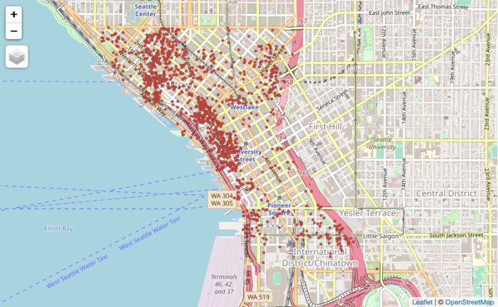
We first narrowed the listings into the boundaries of Downtown Seattle, denoted by both the Zoning Data set and the City Clerks Neighbourhood dataset. From the plot above, it is evident that these listings are unevenly distributed.
Variables and Feature Engineering
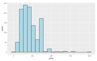
1. Dependent Variable: Price
The histogram plot of the prices in the Downtown area is very much left-skewed.
After removing a listing that is $0 in price, the summary statistics of Airbnb listing prices are as follows:
- Min: $39.00
- 25th percentile: $135.50
- 50th percentile (Mean): $199.00
- 75th percentile: $275.00
- Max: $999.000
2. Independent Variables:
In the Airbnb dataset, the variables which we have chosen to take a deeper look at, screened for multicollinearity and the feature engineering we have done has been summarized in the table below:
| # | Variable | Description of Variable and Wrangling done |
|---|---|---|
The number of guests the listing can accommodate; serves as a proxy to replace the square_area of each listing, which was omitted since more than 80% of the observations were missing | ||
| Feature Engineering: Out of the 157 possible listings found in downtown listings, we categorized the amenities into 3 groups to help with discriminating the prices in Airbnb listings better. This was inspired by GuestReady’s article on the must-haves and ‘wow’ factor extras. We then computed an index value ‘AmenitiesIndex’, which weighs the count of each category of amenities the listings have. The 3 groups are namely; 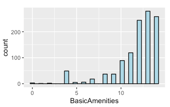 (1) Basic Amenities: Includes essential amenities such as Wifi, Heating, a Laptop friendly work space, Washer etc., including amenities that make up the criteria of what Airbnb defines as the minimal for a ‘Business Travel Ready’ listing. These basic amenities are present in at least 50% of listings  (2) Leisure Amenities: Beyond the basics, the article suggested that guests seeking a ‘home away from home’ comfort would require a few more amenities to make their stay more comfortable; which includes amenities such as cooking basics, a dishwasher, 24 hour check ins, a pool etc. In our categorization, we defined leisure amenities as those present in only 25-50% of listings.  (3) Luxury Amenities: This last group contain amenities and facilities which are more rare in nature, such as a hot tub, lock box, BBQ grill, and having a patio or balcony etc. These amenities are present in around 10-25% of the listings. From these three groupings, our understanding was that luxury amenities would best be able to differentiate the listings in terms of price. However, we cannot discount the presence of the basic and leisure amenities in providing a gauge for price as well. As such, we assigned a weight of 70% to luxury amenities, 20% to leisuire amenities and 10% to basic amenities in formulating the variable AmenitiesIndex. | ||
Categorical variable describing the type of property e.g. Boutique hotel, Condominium, Hostel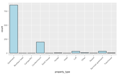 | ||
Categorical variable describing the space which is listed out i.e. Entire home, Private room or Shared room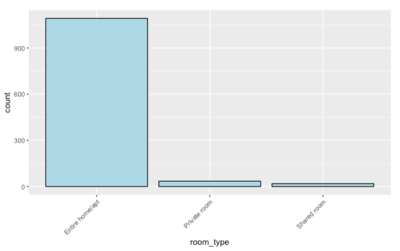 | ||
Number of bathrooms available in the listing | ||
Categorical variable describing the type of bed available e.g Airbed, Couch, Sofa etc. | ||
Numerical variable of the minimum number of nights for booking to be eligible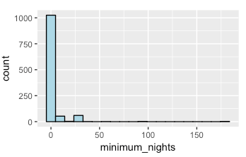 | ||
Numerical variable of the maximum number of nights a guest can book the listing | ||
Categorical variable describing the type of cancellation plan the host has for the listing e.g Strict with 14 day grace period, Super Strict 30 etc. | ||
The neighbourhood which the listing belongs in, spatially joined from City Clerks Neighbourhood data | ||
Numerical variable of the number of reviews the listing has received | ||
Numerical variable of the average rating score received by past guests; of which 235 of 1147 values were missing. Evidently, the distribution was very left skewed. 
| ||
| Date variable showing when the listing’s host joined Airbnb Feature engineering: We created the variable host_experience, which captures the number of days since the host_since to the scrape date.  | ||
Categorical variable describing the frequency of response by the host. Takes on values such as “less than 1 hour” | ||
Binary variable showing if the listing’s host is an Airbnb superhost. A superhost needs to achieve the following:
 | ||
Binary variable showing if the listing’s host has their profile verified | ||
| Numerical variable describing the OpenStreetMap distance required to walk from the listing to the centroid of the following attractions: Seattle Great Wheel, Pike Place Market, Seattle Art Museum, Benaroya Concert Hall, The Seattle Aquarium, Seattle Public Library, Columbia Centre.
These attractions have been grouped together into a centroid value as the correlation matrix showed that there was high collinearity between them. 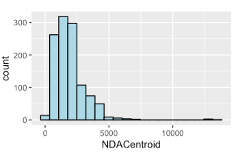 | ||
| Numerical variable describing the OpenStreetMap distance required to walk from the listing to the centroid of the following attractions: Space Needle, Washington State Ferries, Columbia Centre.
These attractions have been grouped together into a centroid value as the correlation matrix showed that there was high collinearity between them.  | ||
Numerical variable describing the OpenStreetMap distance required to walk from the listing to the Klondike Gold Rush attraction |
Project Storyboard
We got our UI inspiration for RShiny Application mainly from The A-maize-ing Corn's RShiny Application (link: https://wiki.smu.edu.sg/18191isss608g1/ISSS608_Group07_Proposal). Their project was also based on Geographically Weighted Regression model and there were many parallels that we could draw and adopt to our project. That was also the first ever RShiny that we ever interacted with and that experience left a lasting impression.
 |
 |

 |
 |

 |

Bearing in mind all points we learnt from The A-maize-ing corn's RShiny application, we decided to try and emulate their design. However, there were a few constraints that we faced.
- We were unfamiliar with RShiny and were worried if we could not deliver what we set out to achieve
- RShiny application development was one the last steps of our project and we were tied down with trying to clean up our code. Timeline was extremely tight!
- At week 10/11, our project's outcome still murky. We initially conceptualised for 'Occupancy Rate' to be our Dependent Variable but we were unable to do it due to data set constraints. Ultimately, we had to tweak our project objective and that was a significant portion of time wasted.
Here are four screenshots of our RShiny application that we conceptualised:
 |
 |

The earlier screenshots were our initial strategy. However, due to time constraints and unfamiliarity with RShiny, we had to abandon some of our design principles. However, we still wanted to deliver on the content points. The key features had to delivered and we prioritised that over the look of our RShiny application. Only when we included all our content points did we then revisit our design principles.

Application Overview

This is how our RShiny Application's front page looks like. There are three main areas that a user can explore. Project Sandbox (under the Overview tab), Point Pattern Analysis to understand the distribution/density of street(s) in Downtown Seattle and Geographically Weighted Regression that allows users to select their most appropriate variables, bandwidth and kernel function to help them determine better listing prices to set!
To find out more about how our application works, look for the 'Business Mafia RShiny Application User Guide' pdf file under the Application tab of our project wiki. Alternatively, click on BusinessMafia Application!
Our Findings
Geographical Accessibility

From our visualisation, it is apparent that most of the darkest spots (dark brown colour) are found between the middle and upper areas of our plot, closer to the coastal areas of Downtown Seattle.
We believe that there are two reasons behind this. Firstly, the attractions found at the top of Downtown Seattle are largely open-air spaces that have capacities in the tens of thousands. The attractions found there are the Washington State Ferries, Space Needle and Olympic Sculpture Park. With close proximity to these places and with these places having high capacities, it is expected that the listings surrounding them tend to have higher accessibility scores.
Secondly, most of the key attractions are found within central of Downtown Seattle. While these places individually do not have capacities as high as the ones above, but by having majority of attractions found within the area, the total capacity of the area is equally large. Hence, it is also expected that listings found within this area should have higher accessibility scores then others.
With our findings, we hypothesize that areas with higher accessibility scores should fetch higher listing prices, given their location superiority.
Spatial Point Pattern Analysis
Quadrat Analysis
The outcome of our quadrat tests produced significant results. Running a simulation of nsim = 2,999, we obtained a p-value of 0.0006667 for all 3 dimensions of quadrats which is lesser than our alpha value of 0.001. Hence, we can confidently reject the null hypothesis of CSR and accept the alternative hypothesis that the distribution of Airbnb listings follow either a regular or cluster pattern.
Kernel Density Estimation
Rescaling the distance of the shapefile to kilometres, we produced the following KDE raster file.

L-Function
After the necessary conversion of a “spatialpointdataframe” (spdf) to a “spatialpoint” (sp) only class, and then a “ppp” object, as well as converting the boundary base map shape file to an “owin” object, we obtained the following point pattern plots in each small neighbourhood (See the first plot below).
From that first plot, International District displays the least clustered distribution of listings amongst the 5 small neighbourhood.
On the other hand, Belltown and Central Business District reflect one of the most clustered patterns. The clustering in Belltown tends to gravitate towards a linear vertical band while the Central Business District shows 2 possible cluster areas – each in the west and north. To derive our statistical results, we then performed the Lest envelope function. The results are seen in the second plot below.
Here is how we interpret the L-function results. The middle dark grey band represents CSR. Its top boundary, known as the upper envelope, represents the 99.9% significance level in our review. Its bottom boundary, known as the lower envelope, is the 0.1% significance level. Any line which falls between the upper and lower envelops represents CSR and so we do not reject the null hypothesis. The key areas we focus in each plot are the points where the black line crosses above or below the upper or lower boundaries. The intersections mark the formation of clusters or regular patterns respectively.
Analysing each plot, we would notice that there is no significant pattern of regular distribution. Each neighbourhood has a different minimum distance of cluster formation and they are mostly very small. As expected, the least clustered region of International District has the largest cluster distance of approximately 20m. And the smallest is Belltown with approximately 2m; a reflection of stronger clustering patterns.


One possible reason for the high listing counts in Belltown (n = 541) is likely attributed to it being the most densely populated neighbourhood in Seattle, Washington and whose rents of residential areas are also low . Sitting on a plot of land that is artificially flattened, it has become a place for popular restaurants, social activities such as nightclubs, bars, art galleries, and an urban environment with new condominium blocks. More so, it is the neighbourhood that is closest to one of the most attractive places in Seattle – the Space Needle. And because Belltown is known for popular streets such as First Avenue, it could explain its clustered pattern of listings mimicking a vertical corridor. These features of low costs, and abundance of tourists features, and an urban atmosphere, makes a strong case for Belltown’s high listing counts.
On the other hand, International district (also known as Chinatown) sees the second lowest number of listing counts (n = 68), with the largest minimum distance for clusters. A possible reason for this lacklustre listing count is possibly because of its unpopularity. According to trip advisor’s ratings and reviews, the location is largely reviewed as being less urbanized and with poor building conditions. In addition, it is situated further away from most attractions. These are possible explanations for its low listing counts.
Geographically Weighted Regression Model
Global Regression Model
After accounting for any potential multi-collinearity between two or more variables which result in unreliable results, a multiple linear regression model was conducted on Price (DV) against the explanatory variables (IV); using the Ordinary Least Square (OLS) regression method.
The variables which are significant at 95% were filtered out to perform a second MLR, which gave rise to a R2 value of 51.81% and an adjusted R2 value of 50.51%. This suggests that without including the geographic location of the listings, the variables explain ~50% of the variation in price.
Local Regression Model
The distribution of local R2 values, the spread of R2 can be attributed to the standard deviation of the gaussian function.

Amongst the variables provided, there are a few which are categorical whilst most are numerical. Studies show that caution needs to be exercised when including categorical data since there is a strong risk of encountering local multicollinearity issues where the categories cluster together spatially . However, as these categorical variables are significant in explaining the variation in prices in the global regression model, we decided to include them in the application, which is only available for kernel functions gaussian and exponential.

From the table above, it is evident that categorical variables such as neighbourhood (e.g. Pike Market, CBD), property type (e.g. condominium, RV), room type (e.g. entire apartment, private room) and type of cancellation policy (e.g. strict 30 days) play a significant role in explaining the variation in prices. In fact, R2 increased by 20% to 50.64% with the inclusion of these variables.


Comparing the R2 plots above, it is evident that the exponential kernel function is, on the whole, more adept at explaining the variation in prices in this local regression model, this can be seen from the lower bound of the R2 values, where the model with exponential kernel function reflects a minimum of 70%, while the gaussian reflects a minimum of 55%.
Additionally, the plots also show a distinctive difference in the spread of R2 values. In the gaussian plot, R2 values tend to take on similar values over a wider distance compared to the exponential kernel function. This can be explained by the difference in the weighting functions used. Comparing the gaussian and exponential curve, the exponential weight function adopts a much steeper decrease compared to gaussian.
Shifting the focus to the Intercept plots, it can be observed that the intercept values are generally on the higher end for listings near to Washington Convention Center, and lower for listings near the pier. This could be justified as Seattle is a magnet for business travellers , and being the largest convention centre in Seattle, listings near this location where business travellers tend to congregate would give it prestige by nature of its location.
Reflecting on our project
 |
 |
Reflections from every team member
Jia Khee:
This was an extremely challenging but immensely gratifying project for me. There were many 'firsts' throughout this journey and I was constantly forced to put on different 'hats' at different point in time, to consider the problem from different angle and think about how best to present a solution. This course was not just about learning analytics. At times I had to put myself in the shoes of an Airbnb host, to think about how they would conduct their business. Another time, I had to think like a UI/UX designer. I had to look into colour schemes, if the colour/design of our logo matches with our project wiki's taskbar. Also, I had to think like a Customer Service Officer - having to try and put myself in the shoes of visitors who were coming down to view our presentation and thinking about the possible questions and doubts they would have. While this project was analytics-based, I learnt from this project that analytics played a major role, but it was not the only area we had to concern ourselves with. To do well, it is equally important that one is able to communicate his/her findings in a simple, non-technical way that everyone will understand. While this project journey has not been easy for me, I am glad that I took on the challenge head on. No regrets!
Chloe:
The basics of information gathering lies in the 5Ws and 1H. For the past 8 semesters in SMU, the Business undergraduate programme led me to focus on the ‘How’ and the ‘Why’. Through our journey in this project, however, I learnt the significance of answering the question ‘Where?’. IS415 Geospatial Analytics has exposed me to an area of analytics I had never imaged to be so extensive in both depth and breadth. I also came to appreciate the applicability of Geospatial Analytics; how it can move business decisions forward and how geospatial visualisations allow for the communication of how patterns and relationships evolve spatially, much more easily. While hands-on exercises and assignments were already challenging, the project took on a whole new level of commitment, research and lots and lots of trial and error.
The project had begun with exploring how different variables affected the demand of a listing. After delving more extensively into data exploration and feature engineering in preparation for the Geospatially Weighed Regression, I had come to realise a key problem: the unreliability of our dependent measure. After realigning our project topic in Week 10 to instead focus on price as the dependent value, the process of feature engineering was reiterated yet again. Despite having many moments of this project journey feeling like it would not come to fruition or meet expectations, I am very glad that the journey had taken the twists and turns that it did, and more importantly that it occurred alongside supportive teammates Bobby and Jia Khee. It had surfaced the importance of data exploration and preparation, and from this journey, I learnt how to work with, interpret, visualize and use spatial data in order to come up with actionable insights in a variety of manners. Moving forward, I am excited to explore more applications of geospatial analytics, especially as the availability of spatial data continues to increase.
Xin Yuan:
This project has been every bit enjoyable and fulfilling as I hoped it would be. It was certainly challenging and time consuming but putting our wits together to practically apply our learnings from class was, in my opinion, a better way to learn; "getting our hands dirty". Working with brilliant friends and guided by a fatherly professor, there are so many takeaways which I have gained - both conceptually and innately. Here are some.
On a technical front, there were many hurdles which i faced. One notable one was the uploading of our application onto the RShiny platform. It being my first time publishing a web based application, I faced many errors. Fortunately, I realised that the error logs was a way I could investigate the issues faced. One problem worth noting was that the usage of '+init=EPSG:32148' was suppose to be '+init=epsg:32148'.
With regard to the concepts, I realised fitting into our project what we've heard alone in class was insufficient. The content covered in class is definitely plentiful but as what Prof Kam says, it's never enough. I slowly understood that the usage of concepts depends tremendously on the contextual problem. It's not about adapting the problem to the concept but the reverse. This helped us manage the use of our concepts more competently.
Lastly, and perhaps my greatest takeaway, is knowing that part of the journey to data science is also accepting (many) painstaking hurdles and troubleshoots to come your way, and being willing to start from scratch if needed. As a team, we've faced so many hurdles together but I was glad we stuck through thick and thin; helping each other all the way to the end. A timely moment to share a quote - "If you can meet with Triumph and Disaster, and treat those two impostors just the same".
Project Timeline
