ISSS608 2017-18 T3 Assign Lim Yee Cheng Data Preparation
|
|
|
|
|
Link to Interactive Visualisation on Tableau Public: https://public.tableau.com/views/ISSS608_201718-T3_AssignmentMC2_LimYeeCheng/AvgValueofContaminantbyLocation?:embed=y&:display_count=yes&publish=yes
Contents
The Data
The data provided for this challenge are as follows:
1) Boonsong Lekagul Waterways Readings which contained several years of water sensor readings from rivers and streams in the preserve, containing the following variables:
- Id: Identification number for the record (only for bookkeeping)
- Value: Measured value for the chemical or property in this record
- Location: Name of the location sample was taken from
- Sample Date: Date sample was taken from the location
- Measure: Chemicals (e.g., Sodium) or water properties (e.g., Water temperature) measured in the record
2) Chemical units of measure in terms of milligram/litre, microgram/litre or degree Celsius
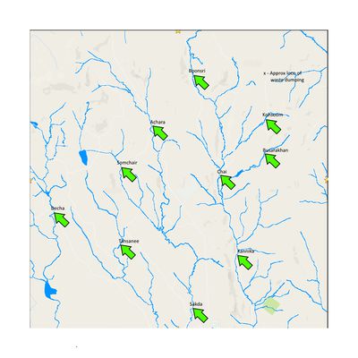
3) A map of the Boonsong Lekagul Waterways with the locations where sensors are placed:
Analysis Tools Used
The tools used for data exploration and preparation were as follows:
1. SAS JMP Pro 14
2. Tableau 2018.1
Data Exploration in JMP Pro 14
The “Boonsong Lekagul Waterways Readings” file was imported to JMP Pro 14. The Univariate Distribution command was then used to get a sense of the data, by producing summary statistics and basic plots of the counts.
The first key observation was that there is a huge disparity in the counts of the various measures:
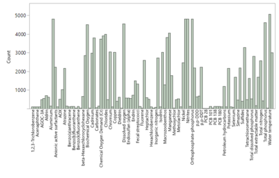
Specifically, the counts ranged from 7 to 5,031, which strongly indicated that there would be huge disparities in the counts along other dimensions, such as location and date, as well.
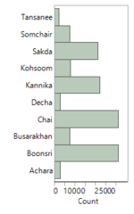
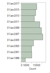
Indeed, disparity was observed in the plots of counts by location and date, as below:
The second observation was that many of the measured values were close to zero. In fact, 25% of the values were 0.6 or below, while the median was 1.86:
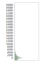
Given that the units of measurement for the chemicals were either milligram/litre (mg/l) or microgram/litre (ug/l), that meant that many of the measures had concentrations too low to be considered as contaminants.
The conclusion from the data exploration in JMP Pro is that, for measures whose values were measured infrequently and/or whose values were too low to be of concern, they should be excluded from the subsequent data visualisation to avoid adding unnecessary and distracting noise.
Data Preparation in Tableau
Firstly, it was necessary to transform the static map of the Boonsong Lekagul Waterways to an interactive one that Tableau could interact with. Reverse-geocoding was used, whereby the relative coordinates of every sampling location were identified within Tableau itself.
An excel file was created with the locations in one column and two empty columns to their right, which would later be filled in with the X and Y coordinates from Tableau. The upper-left, upper-right, lower-left sand lower-right corners were then given values of (0,249), (249,249), (0,0) and (249,0) respectively.
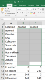
Next, the excel file was imported into Tableau, where point-annotations were manually added to each sampling location. As Tableau automatically calculated the relative X and Y coordinates based on the corner coordinates specified in the excel, I simply had to copy and paste the right values back into the excel file, which then gave me the data necessary for an interactive map in Tableau that visualisations could be added to.
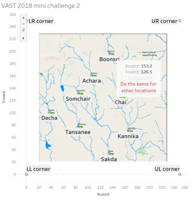
With the inteactive map done, the main “Boonsong Lekagul Waterways Readings” file was imported into Tableau. From the Waterways map, the sampling locations were evidently scattered across different river systems. Hence, within the Data Source pane, the locations were grouped accordingly. The river system closest to the approximate dumping site contained Boonsri, Busarakhan, Chai, Kannika and Kohsoom. The second-closest river system contained Achara, Sakda and Somchair. Decha and Tansanee were the furthest away.

Based on the data exploration previously done in JMP Pro, many of the measures were identified as having values that were measured infrequently and/or having values that were too low to be of concern. Furthermore, some measures were water properties rather than contaminants, such as water temperature. All told, 71 of these irrelevant measures were filtered out within the Data Source pane, using the Data Source Filter, leaving behind 35 measures of significance.
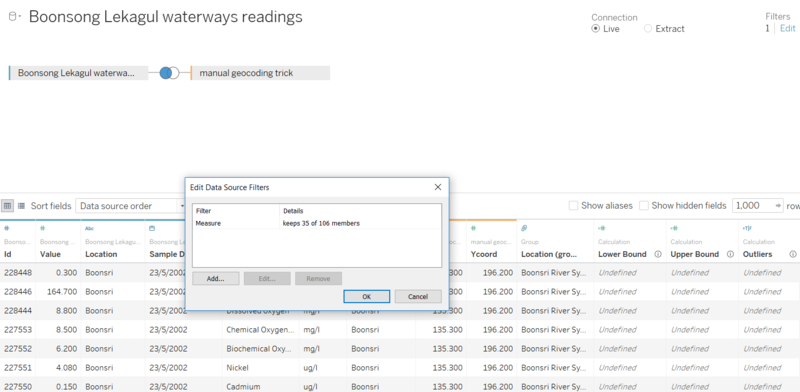
The 35 retained measures:
AGOC-3A, Ammonium, Arsenic, Bicarbonates, Biochemical Oxygen, Cadmium, Calcium, Chemical Oxygen Demand (Cr), Chemical Oxygen Demand (Mn), Chlorides, Chromium, Copper, Dissolved oxygen, Dissolved silicates, Fecal coliforms, Fecal streptococci, Iron, Lead, Macrozoobenthos, Magnesium, Manganese, Methylosmoline, Nickel, Nitrates, Oxygen saturation, Petroleum hydrocarbons, Potassium, Silica (SiO2), Sodium, Sulphates, Total coliforms, Total hardness, Total nitrogen, Total organic carbon, Zinc
The 71 measures that were filtered out:
1,2,3-Trichlorobenzene, 1,2,4-Trichlorobenzene, Acenaphthene, Acenaphthylene, Alachlor, Aldrin, alpha-Hexachlorocyclohexane, Aluminium, Anionic active surfactants, Anthracene, AOX, Atrazine, Barium, Benzo(a)anthracene, Benzo(a)pyrene, Benzo(b)fluoranthene, Benzo(g,h,i)perylene, Benzo(k)fluoranthene, Berilium, beta-Hexaxchlorocyclohexane, Boronm, Carbonates, Cesium, Chlorodinine, Chrysene, Cyanides, Dieldrin, Dissolved organic carbon, Endosulfan (alpha), Endosulfan (beta), Endrin, Fluoranthene, Fluorene, gamma-Hexachlorocyclohexane, Heptachlor, Heptachloroepoxide, Hexachlorobenzene, Indeno(1,2,3-c,d)pyrene, Inorganic nitrogen, Isodrin, Mercury, Methoxychlor, Metolachlor, Naphthalene, Nitrites, Organic nitrogen, Orthophosphate-phosphorus, p,p-DDD, p,p-DDE, p,p-DDT, PAHs, PCB 101, PCB 118, PCB 138, PCB 153, PCB 180, PCB 28, PCB 52, Pentachlorobenzene, Phenanthrene, Pyrene, Selenium, Simazine, Sulfides, Tetrachloromethane, Total dissolved phosphorus, Total dissolved salts, Total extractable matter, Total phosphorus, Trifluralin, Water temperature
