Methods

Rose-crested Blue Pipit: Where are you?

Overview

Methodology

Answers

Conclusions

Tools

Tableau: to do data exploration,visualize data dynamically.

R: to clean data after exploration, and to create visualization that Tableau is not suitable for.

Packages used: tidyverse, lubridate,ggplot2,MASS,viridis.

Python: to process the audio files and visualize the files.

Packages used: os,glob,librosa(librosa.display),numpy,matplotlib.pyplot

Data Exploration and Data Preparation

Data Description

“ALL BIRDS.zip” contain calls and songs from the known birds in the Boonsong Lekagul Wildlife Preserve. These files are MP3 format and are of varying lengths. The name contains an integer that refers to the metadata about the particular bird and audio file in file “AllBirdsv4.csv”.

There are 2081 audio records with 2081 distinctive file ID in AllBirdsv4 csv file.
Among these records, 11.58% are Queenscoat, 10.33% are Orange Pine Plover, and 8.94% are Rose-crested Blue Pipit.
The distribution of vocalization type is 56% call, 37% song, and the rest as call and song together, unknown type, and drumming.
The distribution of sound quality is 32% A, 45% B, 16% C and the rest as D, E, or unknown.
Time has different format (i.e. 9:30 pm, 21:30, 21;30), and the time interval is not constant.
The date of sound collection ranges from 25/07/1983 to 10/03/2018.

Data Exploration with Tableau

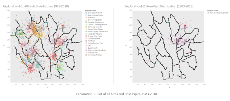
The first thing I did is to check the overall distribution of all birds in all year. The red square is the waste dump site.
Finding is that many bird species have ever lived around the dump site, especially Rose pipit, our object of study.
Since it is cumulative data, it is hard to tell how the distribution changes through years. So the next step is to check the changes over years.

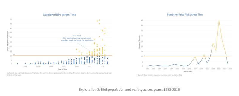
Exploration 2 shows the changes of the bird species variety(number of points) and population of each variety(y value).
It is apparent that the bird species did not become abundant until 2012,and so is the population. Most species reach 10 birds since 2012, including Rose Pipit.
With information collected so far, it is safe to focus on data after year 2012.

Data Cleaning with R

Data cleaning list:
1. Convert file_id to character.
2. Convert X and Y to continuous.
3. Deal with abnormal values in Y col.(found during Exploration stage, shown in Tableau as two null values when plotting X and Y.

4. Standardize levels of Visualization Type variable: all values to upper case, remove redundant space in some rows.

5. Derive a standard date column named "Date_new" and derive Quarter and Season column from Date_New.
6. Export clean data as csv file, named "All_clean"